Sugarcane transportation process modeling by time series approach
F. Afsharnia1*, A. Marzban1, A. Abdeshahi2
1Department of Agricultural Machinery and Mechanization Engineering, Agricultural Sciences and Natural Resources University of Khuzestan, Ahvaz, Iran, I. R. Iran
2Department of Agricultural Economic, Agricultural Sciences and Natural Resources University of Khuzestan, Ahvaz, Iran, I. R. Iran
*Corresponding Author: [email protected] 10.22099/iar.2019.5192
ARTICLE INFO ABSTRACT- Sugarcane is one of the severely perishable crops that is used as raw
material for white sugar production. Sucrose content of the sugarcane which is of high commercial value decreases in quality due to pre-harvest burning, high ambient temperature, kill-to-mill delays as well as microbial contaminations. Delays in sugarcane transportation are the most important risks which can affect the quality and quantity of the product. Delay in milling of the harvested sugarcane is caused by various reasons in agro-industry units including factory downtime, breakdowns of tractors in the waiting line at factory, tractor accident in factory yard and staff shift changes creating long queues. In order to reduce delays, the present study attempted to forecast arrival and service level of tractor drawn carts which transfer burned or cut canes from farm to mill. The univariate ARMA models were applied to forecast arrival and service level. The RMSE and MAPE were also used to evaluate precision of our forecast. The results of models demonstrated that ARMA(4,3) and ARMA(4,2) models are suitable for arrival and service level of tractor drawn carts, respectively. The predicted values trend of arrival, and service level truly reflected the actual values of arrival and service level as well as queue system tendency. The values of MSE, RMSE and MAPE that indicate accuracy of the forecasted carts arrival and service level were relatively low. The estimated models can be used to forecast values of arrival and service levels of tractor drawn carts for subsequent hours during harvest season.
Article history:
Received 20 October 2018 Accepted 19 May 2019 Available online 26 May 2019
Keywords: ARMA Delayed mill Sugarcane Transportation
INTRODUCTION
Sugarcane, as a commercial and versatile crop, plays an important part role in Iran agriculture and industry economy. The market demand for sugarcane will continue to rise due to sucrose production and value-added products such as blackstrap molasses, bagasse,
ethanol, chipboard as well as animal feed, since as one
of the strategic goods is always considered and supported by governments (Le Gal et al., 2008; Chunhawong et al., 2018).
Commercial sugarcane crops (cp69-1062) are grown by furrow irrigation in Sugarcane and Byproducts Development Company, Khuzestan province, Iran. Sugarcane industry is Iran's first-largest agro-based industry providing employment to about 50,000 people and contributing to the growth of the vital rural economy. The Sugarcane and Byproducts Development Company of Khuzestan, as the largest sugar producer in Iran, was able to produce 700 thousand tons of sugar which was half of the country's required sugar. Over the last 45 years, sugarcane cultivation area remained relatively constant in Iran and covered 768,300 hectares in 2016-2017 growing season, while total sugarcane production gradually increased, from around 594,493
in 2016-2017 seasons due to increase in extracting sugarcane juice from the sugarcane sticks from 72.58% in 1971-1972 seasons to 83.48% in 2016-2017 seasons. Furthermore, the sugarcane yield has shown an increase by 102.83% from 24 tons per hectare to 53 tons per hectare in the years 1971-2016 (ISCRTI, 2017).
The harvesting and transportation operations for sugarcane mill are extremely dynamic. As the cane is harvested in the field, the harvester also cuts cane into uniformly sized billets (0.304-0.457 meters) and continuously feeds billets into cart that pulled by a medium powered tractor, usually Massy Freguson 399 (MF-399) tractor. This infield transporter and cart combination runs alongside the harvester during the harvest operations, and when the cart is filled, the tractor runs to mill (sugar factory).
There are many problems causing delays in milling on time. Delays in the billets milling has many reasons in agro-industry companies including sugar mill downtime, tractors failures in the waiting line, accident due to crowd of tractors in yard of the factory and shift changes, all these created quite long queues. The actual occurrence of a long queue in the queuing system is
Afsharnia et al. / Iran Agricultural Research (2018) 37(2) 117-126
118 repair takes more than a day due to the problems of
acquiring replacement parts and the work complicated in repair (Afsharnia et al., 2o13; Afsharnia and Marzban, 2017). So, the amount of time when the tractor operators spend queuing is still very high. The majority of tractor operators in these agro-industries have contract with Sugarcane and Byproducts Development Company to attribute rights and responsibilities between both sides based on the amount of tonnage delivered to the mill. So, they have to wait in a queue prior to unloading their sugarcane at the mill. The tractors unload base on first-come-first-serve. The waiting time for each tractor may take up to 20 hours to complete the handling process, which cause significant increases in costs. These costs could not only include sucrose loss of sugarcane as a result of delay in milling, but also include opportunity cost, accidents costs and the cost of operators servings. Furthermore, under normal conditions, time delay in harvesting sugarcane slightly reduces the amount of commercial sugar mostly due to increase of cane dextran during harvesting to milling which in turn reduces the quality of produced sugar. Clarke (1991) observed that 0.04% of sucrose will decrease at 0.1% of dextran level. Sayed (1972) and later Legendre (1985) concluded that if the burned or cut cane is not crushed within several hours after harvesting, the available sucrose in cane scions will be inverted in the fractured parts of scions by breathing process. Furthermore, cane quality and amount of recoverable sugar could be reduced by loss of injured cells sap and attack of invertase microorganisms to scars.
Queuing system management is a critical component in any sector of business which can reduce the waiting time for operators that are in queues and increase the quality of service of the intended system. The appropriate management decreases the costs and maintains the quality of sugarcane billets. The objective of this study was to combine practical means for forecasting arrival and service level of the sugarcane carts to obtain the best model for the accurate time forecasting when the tractors operators spend in queuing of sugarcane delivering process to mill.
MATERIALS AND METHODS
Data Collection
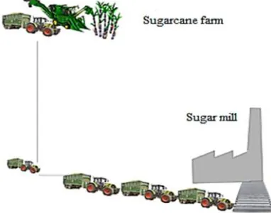
Sugarcane has been widely cultivated agro-industry companies in Khuzestan province, Iran during the last decades. The average of cane harvested was 9000 hectares per year. These companies harvested cane between November and March when rainfall was less frequent and the plant's sugar content was at its highest level. There were 24 sugarcane harvester machine (Austoft 7000), 90 MF399 tractors and 90 carts in these companies. Sugar mill was located near the sugarcane farms at this companies site (Fig.1). The average distance between the farthest sugarcane farms to the sugar mill was 13 km. Based on preliminary observations of these companies, the factory mill
operated and crushed sugarcane billets at 24 hours per day where there was a feed elevator to convey billets for processing plant. The plant was experiencing heavy queues and therefore each cart has to wait in a considerable time for a service to begin. The queuing system in Sugarcane and Byproducts Development Company was a M/M/1 queue in which there was one server and one channel (Arifin et al., 2015). The required data related to arrival and service times of tractors was collected from October 2017 to May 2018 and comprised 56000 observations. Furthermore, factory breakdowns data including conveyors, mill, steam furnace and production hall failures were collected and derived from company records valid in the study region. Data analysis was performed according to the queuing models in the agro-industry unit (Arifin et al., 2015).
Fig. 1. The process of sugarcane stem transportation from farm to factory
Model Description
ARMA (Autoregressive Moving Average) Process
The Autoregressive and Moving Average models (ARMA) often provide actual time series data (Fan and Fan, 2015). The ARMA model integrated a combination of AR and MA into the same equation which is the most general category of models. An ARMA model is merely a stationary series in level of the variable. If the series are not stationary, the Autoregressive Integrated Moving Average model (ARIMA) can be used.
The most general ARMA model simply combines AR and MA Eqs. where p is the order of the autoregressive part and q is the order of the moving average part (Chatfield, 2000) as follows:
= + + + ⋯ + + −
− − ⋯ − (1)
In this formula,
, … … … … . . and … … … … . .
et~ (0, )is white noise with etmutually independent for all t (Thiesson et al., 2004).
Box-Jenkins Methodology
This methodology consist of four phases (Gujarati and Damodar, 2003). For better clarification, the original equation and symbols have been remained unchanged which are as follows;
Model Identification
In modeling phase, it is of prime importance to check whether the series are stationary or not. This needs to be known since the estimation procedure are merely based on stationary series. Stationary in variance and means are two classes of stationary, stationary could be discerned by attending to the graph of the data, which are correlated either as partial correlation coefficient or autocorrelation structure. In cases in which the model is seemed to be non-stationary, differencing the series would be the solution. Some transformation modes such as Log transformation are able to get stationary in variance. In identification phase, obtaining the initial values of the order of non-seasonal and seasonal parameters (p, q, and P, Q) is the next step. One must look for significant autocorrelation and partial autocorrelation coefficients, to find numerical values of abovementioned parameters. It is essential that the sample coefficients of autocorrelation to be good estimates of the population autocorrelation coefficients. However, these estimations could be utilized as an initial guess of iterative steps. Another use of autocorrelation function is to find seasonal component. This happens when the coefficients of autocorrelation at
lags between ‘t’ and ‘t-12’ are significant, otherwise, the
coefficients will not have a significant difference with zero.
Model Estimation
At the previous phase, a few models were temporarily picked. Those models must provide satisfactory representation of the available data. Then, the precise estimates of the model parameters can be obtained by the least squares method which was described by Box and Jenkins (Box and Jenkins, 1976). In our study, data analysis were performed by Eviews 8 and XLSTAT 2016 to find the estimates of related parameters using repetitious procedures.
Diagnostic Checking
Diagnostic checking for model adequacy was the next step when we estimate the parameters by ARMA model. For adequacy model checking, the back forecasting method was used that described as the estimation of xt for t∈ {−M,−M+1,−M+2,...−2,−1}when the following conditions are jointly satisfied, and Autocorrelation Function (ACF) and Partial ACF (PACF) of residuals could be examined. If the residuals were random, the tentatively identified ARMA model would be adequate.
When the residuals of ACF and PACF are random, all their ACF should be within the following range (Jadhav et al., 2017):
±1.96 − 121
Ljung and Box ‘Q’ statistic could be used to test the
autocorrelation of residuals. The autocorrelations of residuals should have a significant different with zero to get significant correlation in the residuals series. So, there is information left in the residuals which should be used in computing forecasts. This can be calculated as follows:
= ( + 2) = ∑ ( − ) (2)
In the above formula h is the considered as the largest lag, n is the observation number and rk is the ACF for lag k. The Q approximately follows a Chi-square distribution with (h-m) degree of freedom. The term 'm' is the number of parameters (p+q+P+Q). Under
H0 the statistic Q asymptotically follows a χ(h)2. For
significance level α, the critical region for rejection of
the hypothesis of randomness is:
> ,
Selection of suitable forecast models was done by
Akaike’s Information Criteria (AIC) and Schwartz
Basic Criteria (SBC). In analyzing of time series AIC and SBC are being used as standard tools for model quality assessment. A variety of models were estimated and the one with lowest AIC and SBC was chosen as best model. The AIC enables us to determine the differencing order (d, D) which is required to obtain stationary and the proper number of AR and MA parameters. The AIC and SBC were calculated as Eqs. (3) and (4):
= ln + 1 + 2 (3)
= log + (4)
In this formula, RSS is the estimated the residual sum of squares,σ2is the estimated MSE 'n' is the total number of observations and 'm' is the sum of estimated parameters (p+q+P+Q). Sometimes SBC is used as instead of AIC (Jadhav et al., 2017).
Strength of a model to predict Ex-ante and Ex-post was verified by Mean Square Error (MSE) as Eq. (5) (Makridakis and Hibbon, 1979; Samarasinghe, 2007; Safa et al., 2015):
= ∑ ( ) (5)
In this formula Yt is the actual output for the i th
value andŶtis the predicted output for the ithvalue, and N is total number of observation.
Root Mean Square Error (RMSE) calculated as another error estimation index using Eq. (6) (Suresh and Priya, 2011):
= ∑ ( ) (6)
Afsharnia et al. / Iran Agricultural Research (2018) 37(2) 117-126
120
= ∑ ( ) × 100 (7)
where, Yt and are actual and predicted valuesو
respectively.
In our study we used the above three test to verify our models. Finally, 70% of data was used for in-sample modeling and 30% of out-of-sample was considered for validation test.
RESULTS AND DISCUSSION
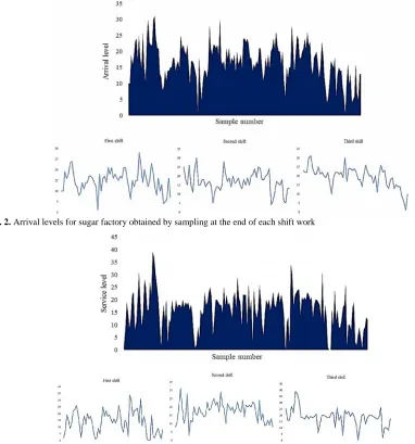
For arrival level changes, as observed on Fig. 2, the behavior of the in-process arrival prior to a sugar factory was provided by observing the queue at the end of each of the three shift work system. In a steady state condition, the trend of queuing system could vary about a mean
level of 16.35 carts and standard deviation of 5.73 carts. Furthermore, according to Fig.2, the mean levels of the first, second and third shifts were 14.7, 16.72 and 19.33 carts, respectively. The arrival level of carts in third shift was higher as compared to other shifts. Out of 24 sugarcane harvester in this company, four or five sugarcane harvesters run at the night, since the arrival level of carts was minimum at the first shift. During every day, the arrival level was gradually increased by increasing the number of active harvesters and consequently increased the amount of harvested crops.
Fig. 3 shows the service level for sugar factory obtained by sampling at the end of each shift with a mean level of 16.82 carts and standard deviation of 7.39 carts. Moreover, according to Fig. 3 the mean service levels of the first, second and third shifts were 13.75, 17.37 and 18.26 carts, respectively.
Fig. 2. Arrival levels for sugar factory obtained by sampling at the end of each shift work
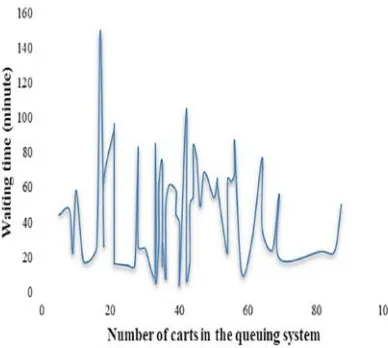
Therefore, it is reasonable to state that the service level was almost agrees with arrival level. Nevertheless, up to 81.6% of carts must wait for more than 30 minutes to discharge billets on feed conveyor. Fluctuation shewing in Fig .4 indicates that waiting time is not related to the number of carts in queue, but it is usually due to breakdowns that occurred in sugar factory equipment. Poor maintenance of the systems can result in the equipment suddenly going dead. Maximum failure of the factory components were related to mill (73%) and feed conveyor (20%), respectively. Only the 25% of total failures were predictable by maintenance experts and the factory scheduled maintenance was only performed for these failures. So, there was not a specific schedule for 75% of other breakdowns that were so unpredictable. This has an impact on the costs and time of agro- industrial units (Afsharnia and Marzban, 2019). The waiting time of carts ranged from 5 to 763 minutes (Fig. 5). The highest mean waiting time of 206.1 minutes per day was observed in the sugar factory yard. The number of carts arriving ranged between 378 and 496 per day, resulted the total unload amounted to 6500 tons day-1. On an average, each cart should wait for 105.6 minutes in discharging queue. Delay in the milling process causes sucrose content degradation as well as dextran, ethanol and oligo saccharides formation in burned or cut canes (Solomon, 2000). Sucrose content of canes lose by 0.0135% per one hour delay (Noroozi, et al., 2015). Accordingly, the total of staled sugarcane would be equal to 1.5 tons per day.
Fig. 4. Waiting time change trend based on number of carts in the queuing system
Fig. 6 shows that the queue length varies during time, it could raise to a high 71 carts after 21 hours, but it could likely decline to 4 carts after 27 hours and then gradually rise to 94 carts after 122 hours and again rise up to 99 after 152 hours. The breakdowns of sugar factory equipments are the main cause of increase in queue length. When the delivery of sugarcane to the mill is not possible, the long queue of tractor drawn carts is created, however the queue reduces as soon as the equipment of sugar factory are repaired. Hourly arrival and service level of tractor drawn carts were
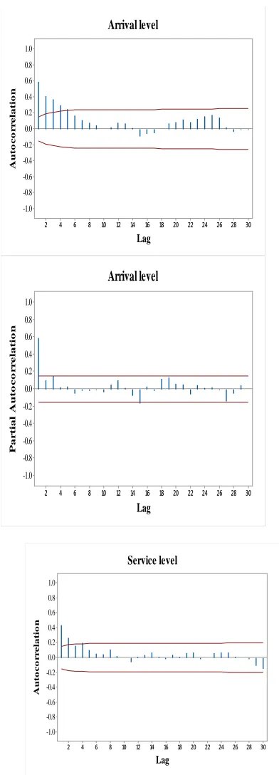
model as outlined in the methodology. Arrival and service level series clearly exhibited stationary as well as lack of seasonality in data. The calculated values of Auto Correlation Function (ACF) and Partial Auto Correlation Function (PACF) of arrival and service level series are shown in Fig. 7 for lags 1-30.
Fig. 5. Waiting time for carts in the queuing system
Fig. 6. The queue length of tractor drawn carts in the system
A glance of the ACF and PACF reveals no evidence of seasonality in the data. The seasonal part of an AR or MA model will be seen in the seasonal lags of the PACF and ACF. Spikes in the ACF (at low lags) indicated non-seasonal MA terms. Spikes in the PACF (at low lags) indicated possible non-seasonal AR terms.
Afsharnia et al. / Iran Agricultural Research (2018) 37(2) 117-126
121 lowest AIC and SBC values to the rest models. After a
repetitious process, the parameters related to the best models were estimated (Table 3).
Fig. 7. Autocorrelation and partial autocorrelation function curve of carts arrival and service level
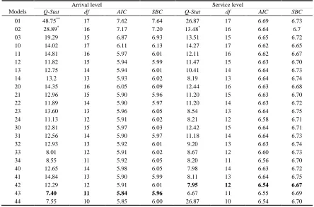
The significance of fitted ARMA models indicated a good fit. Therefore, these coefficients in Table 3 can be used for predicting arrival and service levels. The back forecasting method was used to obtain residuals for checking the model adequacy of the best selected models. The ACF and PACF plots of the residuals for the selected models revealed that there was no autocorrelation between residuals. The Ljung-Box 'Q' statistic was used for model adequacy checking. Non-significant Q-statistic for testing the null hypothesis in which autocorrelations up to lag k equal zero, indicated white noise of series. Therefore, these tests demonstrate that ARMA(4,3) and ARIMA (4,2) models were adequate for forecasting levels of arrival and service, respectively.
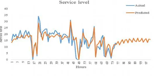
The behavior of Ex-ante and Ex-post forecasts related to arrival and service level of tractor drawn carts are illustrated in Figure 8. The relatively lower values of MSE, RMSE and MAPE compared to other models denoted validity of ex-ante that predicts corresponding to arrival and service level of the tractor drawn carts. There is no study having similar variables and statistical models to our study. The results of analyzing, actual and predicted arrival levels (MSE=4.6, RMSE= 2.14, MAPE= 3.86) revealed that the amplitude of graph fluctuation is generally very high at the first hours of harvesting and then reaches the mean interval level (Fig. 8). At the initial hours of sugarcane harvesting, operation was often irregular due to the low speed at beginning of the work due to calibrating the sugarcane harvesters which did not run on the fields at the last night. The trend of service level graph is illustrated in the Fig. 9 (MSE= 6.6, RMSE= 2.57, MAPE= 7.21).
Table 1. The stationary survey of carts arrival and service level
Test type variable Stationary degree Critical value Calculated value Test result
ADF Arrival level I(0) -2.87 -6.78 Stationary
Service level I(0) -2.87 -8.40 Stationary
Table 2. Models identified for arrival and service level forecast of tractor drawn carts
Models
Arrival level Service level
Q-Stat df AIC SBC Q-Stat df AIC SBC
01 48.75** 17 7.62 7.64 26.87 17 6.69 6.73
02 28.89* 16 7.17 7.20 13.48* 16 6.64 6.7
03 19.29 15 6.87 6.93 13.51 15 6.65 6.72
10 14.02 17 6.11 6.13 14.27 17 6.62 6.65
11 14.81 16 5.97 6.01 12.11 16 6.62 6.67
12 11.82 15 5.94 5.99 11.47 15 6.63 6.70
13 12.75 14 5.94 6.01 10.41 14 6.64 6.73
14 13.2 13 5.93 6.02 8.19 13 6.64 6.74
20 14.35 16 6.05 6.09 12.44 16 6.63 6.68
21 12.96 15 5.90 5.96 11.20 15 6.63 6.70
22 11.89 14 5.90 5.97 11.20 14 6.63 6.72
23 13.60 13 5.96 6.05 8.54 13 6.64 6.75
24 11.13 12 5.91 6.02 8.21 12 6.58 6.71
30 12.81 15 5.97 6.03 12.42 15 6.64 6.71
31 12.56 14 5.90 5.97 11.18 14 6.64 6.73
32 12.93 13 5.92 6.01 9.20 13 6.63 6.74
33 8.01 12 5.91 6.02 8.67 12 6.60 6.73
34 8.55 11 5.92 6.05 8.20 11 6.56 6.70
40 12.65 14 5.98 6.05 7.98 14 6.63 6.72
41 14.84 13 5.90 5.99 8.11 13 6.64 6.75
42 12.29 12 5.91 6.01 7.95 12 6.54 6.67
43 7.40 11 5.84 5.96 6.67 11 6.55 6.69
44 7.55 10 5.85 6.00 26.87 10 6.54 6.70
Table 3. Summary of the statistical parameters of the best fitted ARIMA models on waiting time
Arrival level Service level
Coefficient SE t value Coefficient SE t value
AR1 1.48 0.06 21.91** 0.84 0.07 10.81**
AR2 -0.76 0.12 -6.08** -0.93 0.09 -9.59**
AR3 -0.16 0.12 -4.31* 0.29 0.093 3.11**
AR4 0.16 0.07 2.33* 0.13 0.072 2.86*
MA1 -1.03 0.09 -11.24** -0.47 0.014 -32.47**
MA2 0.32 0.14 2.31* 0.97 0.009 100.15**
MA3 0.45 0.09 4.79** - -
-Constant 17.13 0.86 19.89** 16.41 1.06 15.37**
Afsharnia et al. / Iran Agricultural Research (2018) 37(2) 117-126
124 Fig. 9. Actual and predicted values of service level
The curve in Fig.9 illustrated that instability was retained and oscillations occurred within service interval time. The unloading of tractor drawn carts terminates in sugarcane factory equipment failure time. In other words, when the factory equipment brake down, the delivery of sugarcane billets to sugar factory was stopped. The service level of tractor drawn carts attained higher level after 20 hours at 34 cart per hour and reached the lowest service level of 0 cart per hour after 16 hours. It is clear that the graph oscillations of service level were higher compared to the arrival level. According to failure data, the most problems refers to sugar factory breakdowns. So, the failures of harvesters as well as tractors which used to draw the carts can be ignored.
CONCLUSIONS
The predicted arrival and service level of tractor drawn carts were nearly identical to actual values with very
good validation as demonstrated by the relatively low values of MSE, RMSE and MAPE. Therefore, the ARMA model serves as a reliable method to predict the magnitude of arrival and service level. The results of models fit demonstrated that ARMA (4,3) and ARMA (4,2) models were suitable for estimating arrival level and service level of tractor drawn carts, respectively. The trends of predicted values of arrival and service level truly reflected the actual values as well as queue system tendency. The identified models which can be used to forecast values for arrival and service level of tractor drawn carts are developed for subsequent hours at harvest season.
ACKNOWLEDGEMENTS
The authors would like to acknowledge Iran's National Elites Foundation for financial support related to Agricultural and Biological System Analysis research core of Agricultural Sciences and Natural Resources University of Khuzestan.
REFERENCES
Afsharnia, F., Asoodar, M. A., Abdeshahi, A., & Marzban, A. (2013). Failure rate analysis of four agricultural tractor models in southern Iran. Agricultural Engineering International: CIGR Journal, 15(4), 160- 170.
Afsharnia, F., & Marzban, A. (2017). The effect of usage and storing conditions on John Deere 3140 tractor failures in Khuzestan province, Iran. Journal of Biosystems Engineering, 42(2), 75-79.
Afsharnia, F., & Marzban, A. (2019). The risk analysis of sugarcane stem transportation operations delays using the FMEA-ANP hybrid approach. Journal of Agricultural Machinery, 9(2), 481-496.
Iranian Sugarcane and Byproduct Research and Training Institute (ISCRTI). (2017). Sugar cane factories laboratory guidelines. Khuzestan: Sugarcane Development Company and Subsidiary Industries annals Arifin, M. Z., Probowati, B. D., & Hastuti, S. (2015). Applications of Queuing Theory in the Tobacco Supply.
Agriculture and Agricultural Science Procedia, 3, 255-261.
Box, G. E., & Jenkins, G. M. (1976). Time series analysis: Forecasting and control San Francisco. California: Holden-Day.
Chatfield, C. (2000). Time-series forecasting (1st ed). UK: Chapman and Hall/CRC.
Chunhawong, K., Chaisan, T., Rungmekarat, S. & Khotavivattana, S. (2018). Sugar industry and utilization of its by-products in Thailand: an overview. Sugar Tech, 20(2), 111-115.
Clarke, S. J. (1991). Losses associated with cane yard operations and cane washing. In Proceedings of the annual congress-South African Sugar Technologists' Association, 95, 131-144.
models. Journal of Advanced Management Science, 3(3), 203-210.
Farjam, A., Omid, M., Akram, A. & Fazel, Niari. Z. (2014). A neural network based modeling and sensitivity analysis of energy inputs for predicting seed and grain corn yields. Journal of Agricultural Science and Technology, 16, 767-778.
Gujarati, N. & Damodar. (2003). Basic econometric. New Delhi: McGraw-Hill.
Jadhav, V., Chinappa Reddy, B. V., Gaddi, G. M., & Kiresur, V. R. (2017). Exploration of different functional forms of growth models: a censorious analysis with reference to horticultural sector in Karanataka. International Journal of Tropical Agriculture, 34(4), 1107-1116.
Le Gal, P.Y., Lyne, P.W., Meyer, E., & Soler, L.G. (2008). Impact of sugarcane supply scheduling on mill sugar production: A South African case study. Agricultural systems, 96(1-3), 64-74.
Makridakis, S., & Hibbon, M. (1979). Accuracy of forecasting: An empirical investigation. Journal of the Royal Statistical Society. Series A (General), 142 ( 2), 97-145.
Noroozi, S., Asoodar, M. A., Marzban, A., & Moradi Telavat, M. R. (2015). Sensitivity comparison of the sugarcane mill
delay in Iran. Green sugar cane is more sensitive or burned Elixir Agriculture, 85, 34378-34385.
Safa. M., Samarasinghe, S., & Nejat, M. (2015). Prediction of wheat production using artificial neural networks and investigating indirect factors affecting it: case study in Canterbury province, New Zealand. Journal of Agricultural Science and Technology, 17, 791-803. Samarasinghe, S. (2007). Neural networks for applied
sciences and engineering: from fundamentals to complex pattern recognition. Boca Raton: Auerbach, FL.
Sayed, G. E. (1972). Changes in the sugar components of cane during growth and processing, Ph. D. Thesis, College of Agriculture Library, University of Assiut.
Solomon, S. (2000). Post-harvest cane deterioration and its milling consequences. Sugar Tech, 2(1&2), 1-18. Suresh, K. K., & Priya, S. K. (2011). Forecasting sugarcane
yield of Tamilnadu using ARIMA models, Sugar Tech, 13(1), 23-26.
126
هﺪﯿﮑﭼ ﺮﮑﺷ ﺪﯿﻟﻮﺗ ياﺮﺑ مﺎﺧ داﻮﻣ ترﻮﺻ ﻪﺑ ﻪﮐ ﺖﺳا ﺮﯾﺬﭘدﺎﺴﻓ تﺪﺷ ﻪﺑ تﻻﻮﺼﺤﻣ زا ﯽﮑﯾ ﺮﮑﺸﯿﻧ
ﯽﻣ رﺎﮑﺑ ﺪﯿﻔﺳ ﺮﯿﺧﺄﺗ ،ﻂﯿﺤﻣ يﻻﺎﺑ يﺎﻣد ،ﺖﺷادﺮﺑ زا ﻞﺒﻗ نﺪﻧازﻮﺳ ﻞﯿﻟﺪﺑ زرﺎﮐﺎﺳ يرﺎﺠﺗ ﻊﺒﻨﻣ ﻦﯾا .دور
و بﺎﯿﺳآ رد ﻦﯿﻤﻫ
ﯽﮔدﻮﻟآ رﻮﻃ ﯽﻣ ﺖﯿﻔﯿﮐ ﺖﻓا رﺎﭼد ﺖﻋﺮﺳ ﻪﺑ ﯽﺑوﺮﮑﯿﻣ يﺎﻫ
ﻢﻬﻣ زا ﯽﮑﯾ .دﻮﺷ ﻦﯾﺮﺗ
ﮏﺴﯾر ﯽﻣ ﺪﻨﯾآﺮﻓ ﻦﯾا رد ﻪﮐ ﺖﺳا ﯽﺗاﺮﯿﺧﺄﺗ ﺮﮑﺸﯿﻧ ﻞﻘﻧ و ﻞﻤﺣ يﺎﻫ ار لﻮﺼﺤﻣ ﺖﯿﻤﮐ و ﺖﯿﻔﯿﮐ ﺪﻧاﻮﺗ
ﯽﺑاﺮﺧ ﻪﻠﻤﺟ زا ﯽﻔﻠﺘﺨﻣ ﻞﯾﻻد ﻪﺑ هﺪﺷ ﺖﺷادﺮﺑ ﺮﮑﺸﯿﻧ ندﺮﮐ بﺎﯿﺳآ رد ﺮﯿﺧﺄﺗ .ﺪﻫد راﺮﻗ ﺮﯿﺛﺄﺗ ﺖﺤﺗ ،ﻪﻧﺎﺧرﺎﮐ و ﺖﺸﮐ رد ﺖﻔﯿﺷ ﺮﯿﯿﻐﺗ و ﻪﻧﺎﺧرﺎﮐ ﻂﯿﺤﻣ رد ﺎﻫرﻮﺘﮐاﺮﺗ فدﺎﺼﺗ ،ﻒﺻ رد يﺎﻫرﻮﺘﮐاﺮﺗ ﯽﺑاﺮﺧ
ﺖﻌﻨﺻ ﯽﻣ دﻮﺟﻮﺑ ﺎﻫ ﯽﻣ ﯽﻧﻻﻮﻃ ﯽﻔﺻ دﺎﺠﯾا ﺐﺒﺳ ﻪﮐ ﺪﯾآ
.ددﺮﮔ ﻦﯾا زا ﻪﺑ ﺪﯾدﺮﮔ شﻼﺗ ﺶﻫوﮋﭘ ﻦﯾا رد ،ور
ﺶﯿﭘ يﺮﺳ زا هدﺎﻔﺘﺳا ﺎﺑ ﺮﮑﺷ ﺪﯿﻟﻮﺗ ﻪﻧﺎﺧرﺎﮐ ﻪﺑ ﺮﮑﺸﯿﻧ لﻮﺼﺤﻣ ﻞﯾﻮﺤﺗ ﻒﺻ ﻢﺘﺴﯿﺳ ﯽﻨﯿﺑ ﯽﻧﺎﻣز يﺎﻫ
ﻪﻨﯿﻣز ﺎﺗ دﻮﺷ ﻪﺘﺧادﺮﭘ .ددﺮﮔ ﻢﻫاﺮﻓ نآ يزﺎﺴﻬﺑ يﺎﻫ
لﺪﻣ
ARMA
ﺶﯿﭘ ﺖﻬﺟ خﺮﻧ و دورو خﺮﻧ ﯽﻨﯿﺑ
ﺺﺧﺎﺷ و ﺪﺷ ﻪﺘﻓﺮﮔ رﺎﮑﺑ ﺮﮑﺸﯿﻧ ﻞﻤﺣ يﺎﻫرﻮﺘﮐاﺮﺗ ﺲﯾوﺮﺳ يﺎﻫ
RMSE
و
MAPE
ﯽﺑﺎﯾزرا ﺖﻬﺟ
ﺶﯿﭘ ﺖﻗد لﺪﻣ شزاﺮﺑ ﺞﯾﺎﺘﻧ .ﺪﻧﺪﺷ هدﺎﻔﺘﺳا ﯽﻨﯿﺑ لﺪﻣ ﺐﯿﺗﺮﺗ ﻪﺑ ﻪﮐ داد نﺎﺸﻧ ﺎﻫ
يﺎﻫ
ARMA(4,3)
و
ARMA(4,2)
ﺶﯿﭘ ﺮﯾدﺎﻘﻣ ﺪﻧور .ﺪﻧدﻮﺑ ﺐﺳﺎﻨﻣ ﯽﻧ ﻞﻤﺣ يﺎﻫرﻮﺘﮐاﺮﺗ ﺲﯾوﺮﺳ خﺮﻧ و دورو خﺮﻧ ياﺮﺑ
-ﯽﻨﯿﺑ لﺪﻣ ﻦﯾا دﺮﺑرﺎﮐ ﺎﺑ .دﻮﺑ ﻖﺒﻄﻨﻣ ﯽﻌﻗاو ﺮﯾدﺎﻘﻣ ﺮﺑ ﯽﺑﻮﺧ ﻪﺑ ﺲﯾوﺮﺳ خﺮﻧ و دورو خﺮﻧ هﺪﺷ ﻪﻌﺳﻮﺗ يﺎﻫ
ﺶﯿﭘ ﺮﯾدﺎﻘﻣ ،ﻪﺘﻓﺎﯾ ﯽﻣ ار هﺪﺷ ﯽﻨﯿﺑ
ﻮﺑ تاﺮﯿﺧﺄﺗ زا و دﺮﺑ رﺎﮑﺑ ﺮﮑﺸﯿﻧ ﺖﺷادﺮﺑ ﻞﺼﻓ ﻪﯿﻘﺑ ياﺮﺑ ناﻮﺗ دﻮﺟ
ﯽﻣ لﻮﺼﺤﻣ زا يدﺎﯾز ﺮﯾدﺎﻘﻣ نﺪﺷ ﻊﯾﺎﺿ ﺐﺟﻮﻣ ﻪﮐ هﺪﻣآ .ﺖﺳﺎﮐ دﻮﺷ
ﻪﻟﺎﻘﻣ تﺎﻋﻼﻃا
:ﻪﻟﺎﻘﻣ ﻪﭽﺨﯾرﺎﺗ
:ﺖﻓﺎﯾرد ﺦﯾرﺎﺗ 28
/ 7 / 1397
:شﺮﯾﺬﭘ ﺦﯾرﺎﺗ 29
/ 2 / 1398
:ﯽﺳﺮﺘﺳد ﺦﯾرﺎﺗ 5
/ 3 / 1398
:يﺪﯿﻠﮐ يﺎﻫ هژاو ARMA
ندﺮﮐ بﺎﯿﺳآ رد ﺮﯿﺧﺄﺗ ﺮﮑﺸﯿﻧ ﻞﻘﻧ و ﻞﻤﺣ ناﺮﯾا يزروﺎﺸﮐ تﺎﻘﯿﻘﺤﺗ
117 -126
لﺪﻣ
يزﺎﺳ
ﺪﻨﯾآﺮﻓ
ﻞﻤﺣ
ﺮﮑﺸﯿﻧ
ﺎﺑ
هدﺎﻔﺘﺳا
زا
هﺎﮔﺪﯾد
يﺮﺳ
يﺎﻫ
ﯽﻧﺎﻣز
ﺎﯿﻧرﺎﺸﻓا ﻪﻤﻃﺎﻓ
* 1
،
نﺎﺑزﺮﻣ ﻦﯿﺸﻓا
1
،
ﯽﻫﺎﺷ ﺪﺒﻋ سﺎﺒﻋ
2
1
هوﺮﮔ ﯽﺳﺪﻨﻬﻣ ﻦﯿﺷﺎﻣ ،زاﻮﻫا ،نﺎﺘﺳزﻮﺧ ﯽﻌﯿﺒﻃ ﻊﺑﺎﻨﻣ و يزروﺎﺸﮐ مﻮﻠﻋ هﺎﮕﺸﻧاد ،نﻮﯿﺳاﺰﯿﻧﺎﮑﻣ و يزروﺎﺸﮐ يﺎﻫ .ناﺮﯾا .ا .ج
2
هوﺮﮔ يزروﺎﺸﮐ دﺎﺼﺘﻗا مﻮﻠﻋ هﺎﮕﺸﻧاد ،
زاﻮﻫا ،نﺎﺘﺳزﻮﺧ ﯽﻌﯿﺒﻃ ﻊﺑﺎﻨﻣ و يزروﺎﺸﮐ ،
.ناﺮﯾا .ا .ج
*