Minimum-Weight Link-Disjoint Node-“Somewhat
Disjoint” Paths
Jose Yallouz, Ori Rottenstreich, P´eter Babarczi, Avi Mendelson and Ariel Orda
Abstract—Network survivability has been recognized as an issue of major importance in terms of security, stability and prosperity. A crucial research problem in this context is the identification of suitable pairs of disjoint paths. Here, “disjointness” can be considered in terms of either nodes or links. Accordingly, several studies have focused on finding pairs of either link or node disjoint paths with a minimum sum of link weights. In this study, we investigate the gap between the optimal node-disjoint and link-disjoint solutions. Specifically, we formalize several optimization problems that aim at finding minimum-weight link-disjoint paths while restricting the number of its common nodes. We establish that some of these variants are computationally intractable, while for other variants we establish polynomial-time algorithmic solutions. Finally, through extensive simulations, we show that, by allowing link-disjoint paths share a few common nodes, a major improvement is obtained in terms of the quality (i.e., total weight) of the solution.
Index Terms—link-disjoint paths, survivable routing, selective common nodes, minimum-weight paths, Bellman-Ford
I. INTRODUCTION A. Background
Survivability, i.e. the capability of the network to maintain service continuity in the presence of failures, has been con-sidered as a major challenge for the networking community.
Protection is a widely employed recovery scheme for coping with network failures where a backup path is provided for each established active path [1]. Specifically, pre-failure actions are performed in advance, thus pre-establishing a backup path for any active path and providing protection from any possible failure. The path calculation time might be a major factor for survivability, turning the protection scheme into a favorable approach for a fast recovery time. Indeed, the protection scheme has been considered as a de-facto feasible approach for satisfying the requirements of various standards [2] [3], in which recovery from a single failure must be performed within
50 ms. Moreover, the employment of this scheme can be also utilized for load balancing and security [4].
A fundamental problem in the context of protection schemes is the identification of a pair of disjoint paths, thus providing A preliminary version of this article appeared in the IEEE International Conference on Network Protocols (ICNP) ’16, Singapore, November 2016. Jose Yallouz, Avi Mendelson and Ariel Orda are with the department of Electrical Engineering, Technion, Israel Institute of Technology (e-mail: [email protected],{mendlson@ee, ariel@ee}.technion.ac.il). Ori Rotten-streich is with the department of Computer Science, Princeton University (e-mail: [email protected]). P´eter Babarczi is with MTA-BME Future Internet Research Group, Budapest University of Technology and Economics (BME) (e-mail: [email protected]).
protection against a single failure in the network. Usually, such a pair of paths needs to satisfy some quality (a.k.a. “Quality of Service - QoS”) requirement, which is typically quantified by the sum of some link weights. Accordingly, several studies have proposed algorithmic schemes for finding a fully disjoint pair of paths between a source and a destination that minimize the sum of the link weights [5], [6]. “Disjointness” can be considered either in terms of links or nodes. We note that a link-disjoint pair of paths might contain severalcommon nodes, whereas the node-disjoint solution is a special case of link-disjointness with no common nodes.
From a practical perspective, common nodes along an es-tablished link-disjoint pair of paths might have either (or both) beneficial or detrimental implications. For instance, in cases that the recovery time is critical, the traffic might be retrans-mitted from the closest common node to the faulty link rather than from the source. Another example is the implementation of an encoding scheme in a specific set of common nodes along the link disjoint pair of paths. However, in case of faulty nodes, a common node becomes asingle point of failure. Accordingly, the detrimental and beneficial effects of common nodes can be considered together by allowing (or, alternatively, requiring) that the pair of link-disjoint paths would share a bounded number of common nodes.
an optimal second link-disjoint path given a selection of the first path. Finally, in Section VII, by employing the established algorithmic schemes, we are able to study the gap between the optimal node-disjoint and the optimal link-disjoint solution through extensive simulations.
B. Related Work
An important property of graph connectivity is provided by Menger’s theorem [7], which states that the size of the mini-mum edge cut fromsandt is equal to the maximum number of pairwise link-disjoint paths from s to t. This result was extended to the well-known max-flow min-cut theorem [8]. A simple method for finding link-disjoint paths would implement a maximum flow algorithm fromstotsetting the capacity to1
in all links. However, for many applications, the quality of the solution, e.g. delay or cost, is also an important requirement, giving rise to several optimization problems. The most popular variant is the problem of finding link-disjoint paths between a source and a destination such that the sum of the weights of all the paths’ links is minimized. This problem can be solved in polynomial-time by the well-known Suurballe’s algorithm [5], [6]. However, other objective functions might be considered as well. In [9], the problem of finding link-disjoint paths minimizing the weight of the longest path was proved to be NP-Hard, while Suurballe’s algorithm provides a2-approximation. In [10], the minimization of the shorter path was addressed and proved to be strongly NP-Hard. Next, in [11], the problem of finding a link-disjoint pair of paths that minimizes the total cost of the paths under a constraint imposed by a second weight metric has been considered. This problem was proved to be NP-Hard and a bi-criteriaO(1 +1r,1 +r) approximation for any r ≥0 was proposed. Recently, in [12], an improved constant approximation ratio of (1,2) was achieved.
The present study is somehow related to the concept of
tunable survivability which offers a milder and more flexible approach to the rigid requirement of link-disjoint paths by also considering paths containing common links [13]–[15]. These works first focused on “bottleneck” QoS [13] metrics, then con-sidered the harder class of “additive” QoS [14], while extended in the context of broadcasting through spanning trees [15].
II. MODELFORMULATION
Anetworkis represented by a directed graphG(V, E), where V is the set of nodes andE is the set of links. We denote the size of these sets as|V|=N and|E|=M, respectively. Each link e ∈E is assigned with a positive weight we ∈ R+ that
represents an additive QoS target, e.g. cost or delay. Apathis a finite sequence (ordered set) of nodes π=< s0, s1, ..., sh>
such that si ∈ V (for i ∈ [0, h]) and (si, si+1) ∈ E (for i∈[0, h−1]). A path issimpleif its nodes are distinct. Unless explicitly stated, the termpathis used for a simple path. Along the paper, a link and a path between nodesuandvcan be also represented byu→v andu v, respectively.
A link is classified as eitherfaultyoroperational: it becomes faulty upon a temporary fault and remains to be such during all
the fault period, otherwise it is operational. Failures can occur in every link. Likewise, we say that a pathπis operationalif it has no faulty link, i.e., for eache∈π, linkeis operational; otherwise, the path is faulty.
We adopt the widely employed single link failure model, which has been the focus of various studies, e.g. [10], [16], [17], [18]. Although multiple failures might occur in the network, this model aims at focusing on the most common failure event in which a single link is faulty. Considering this model, a common approach for failure protection is the usage of a pair of (fully) link-disjoint paths between given source and destination nodes.
Definition 2.1:(Link-disjoint Path Pair) Given are a network G(V, E), a source nodes∈V and a destination nodet∈V. A
link-disjoint path-pair(π1, π2)is a pair of paths between these nodes with no common links.
While two paths must be link-disjoint to guarantee surviving any single link failure, they still might share common nodes.
Definition 2.2: (Common Node) Given alink-disjoint path-pair (π1, π2)between a source node s∈V and a destination nodet∈V, acommon nodeof(π1, π2)is a node, other than the source and destination, that belongs to both paths, i.e. a node in{v∈V\ {s, t}|v∈π1 andv∈π2}. We defineC(π1, π2)as the number of common nodes of(π1, π2).
Accordingly, anode-disjoint path-pair(π1, π2)is a pair of link-disjoint paths between these nodes with no common nodes, i.e.
C(π1, π2) = 0.
Often, the weight of a path is defined as the sum of its link weights [19]. This can describe, for instance, the total cost or delay along the path. Generally, we would prefer paths with smaller weights. Since a link-disjoint path-pair is composed of two paths, there are several possibilities to define its weight based on its link weights. We adopt the classical metric which considers the aggregate (total) weight of the two paths (e.g., [5], [6], [16]). This metric accounts for the “average quality” of the paths, and is also suitable in cases where the incorporation of each link in either path incurs some “cost” (e.g., maintenance cost).
Definition 2.3:Given a network G(V, E)and a link-disjoint path-pair(π1, π2), itsweight W(π1, π2)is defined as the sum of weights of the links of its two paths, i.e., W(π1, π2) = P
e∈π1∪π2we = P
e∈π1we + P
e∈π2we. Accordingly, we
define a weight-shortest link-disjoint path-pair between two nodesu∈V andv∈V as a link-disjoint path-pair inG(V, E)
with minimum weight betweenuandv.
Among the different weight-shortest link-disjoint path-pairs, we might have to cope with different restrictions on the number of common nodes, resulting in the following optimization problems.
path-pair(π1, π2)such that:
min W(π1, π2)
s.t. C(π1, π2)≤k.
Problem 2.2: Minimum Weight Link Disjoint Paths re-stricted Tight Bound Common Nodes (MWLD-Tight-BCN) Problem: Given are a networkG(V, E), a source nodes∈V, a destination node t∈V and an integerk. Find a link-disjoint path-pair (π1, π2)such that:
min W(π1, π2)
s.t. C(π1, π2) =k.
Problem 2.3: Minimum Weight Link Disjoint Paths re-stricted Lower Bound Common Nodes (MWLD-Lower-BCN) Problem: Given are a networkG(V, E), a source nodes∈V, a destination node t∈V and an integerk. Find a link-disjoint path-pair (π1, π2)such that:
min W(π1, π2)
s.t. C(π1, π2)≥k.
In the sequel, we will prove that the MWLD-Tight-BCN and the MWLD-Lower-BCN problem versions are NP-Hard, while for the MWLD-Upper-BCN problem we shall establish a polynomial-time solution.
III. MWLD PROBLEMSHARDNESS
In this section, we will prove the complexity of two problem variants, namely MWLD-Tight-BCN and MWLD-Lower-BCN.
A. MWLD-Tight-BCN Intractability
We start by proving that MWLD-Tight-BCN is NP-Hard through a reduction from the2-Disjoint Paths (NP-Hard) Prob-lem [20], where, for a given (unweighted) graph G(V, E)and four distinct nodes s1, t1, s2 and t2, we aim to find2 disjoint pathsΠ1andΠ2between(s1, t1)and(s2, t2), respectively. The complexity of different versions of the problem (Gis directed or undirected, and Π1 and Π2 are link- or node-disjoint) has been investigated in [21]. Shiloach presented a polynomial-time solution for the 2-(node-)disjoint paths problem in undirected graphs [22], while Tholey [23] further improved the time complexity of this algorithm. However, the 2-Disjoint Paths Problem remains NP-complete in directed graphs [20] for both the link- and disjoint case [23]. We will refer to the node-disjoint problem in directed graphs as 2-NDPP.
We proceed to define a decision version of the MWLD-Tight-BCN problem and the 2-NDPP problem, respectively.
• Given are a directed network G(V, E) with positive link
weights we ∈ R+, two distinct nodes s, t, a positive
integer k and a positive value l. Is there a link-disjoint path-pair(π1, π2)betweensandtsuch thatC(π1, π2) =k andW(π1, π2)≤l?
• Given are a directed network G(V, E) and four distinct nodess1, t1, s2andt2. Are there2node-disjoint pathsΠ1 andΠ2between (s1, t1)and(s2, t2), respectively?
G s
v s1
s2
t2 t1
[image:3.612.372.511.57.145.2]t
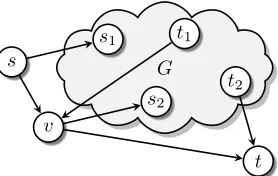
Fig. 1. Polynomial-time reduction of2-NDPP (2-LDPP) to MWLD-Tight-BCN (MWLD-Lower -BCN).
Next, we show that the MWLD-Tight-BCN problem is NP-complete even fork= 1.
Theorem 3.1: The MWLD-Tight-BCN problem for
C(π1, π2) = 1is NP-complete.
Proof: Clearly, MWLD-Tight-BCN is in NP, since for a given link-disjoint path-pair (π1, π2), we can polynomially check whether W(π1, π2)≤l andC(π1, π2) = 1by summing its link weights and counting its common nodes, respectively.
We proceed to prove that the MWLD-Tight-BCN problem for C(π1, π2) = 1 is NP-Hard by providing a polynomial-time reduction from the 2-NDPP (NP-Hard) problem, i.e. 2-NDPP
p MWLD-Tight-BCN. Assume we are given an instance of
the 2-NDPP problem, that is, a directed graph G(V, E) and four distinct nodes s1, t1, s2 and t2. In the polynomial-time reduction, we create a directed graphG1(V1, E1), whereV1=
V ∪ {s, t, v}, where sandtdenote the source and destination node of the MWLD-Tight-BCN problem, respectively, while E1=E∪ {(s, s1),(s, v),(t1, v),(v, s2),(v, t),(t2, t)}. We set
∀e ∈E1 :we = 1, l =Pe∈E1we andk = 1. This auxiliary
graphG1(V1, E1)is illustrated in Fig. 1.
Next, we will demonstrate that the MWLD-Tight-BCN prob-lem in G1 is solvable, i.e., there is a link-disjoint path-pair
(π1, π2) from s to t with exactly one node in common and W(π1, π2)≤l iff 2-NDPP is solvable in G.
(⇒) First, note that the single common node inG1 for any MWLD-Tight-BCN solution must be v. This is because ifπ1 and π2 have the single common node w inside G, i.e., π1 = s → s1 w t2 → t and π2 = s → v → s2 w t1 →v →t, then π2 is a non-simple path. Furthermore, note that the segmentsΠ1 =s1 t1 andΠ2 =s2 t2 must be part of the MWLD-Tight-BCN solution, as otherwise π1 and π2 do not have a node in common (i.e.,π1=s→v→t and π2 =s→s1 t2→t). Finally, either the paths Π1 and Π2 are part of the same link-disjoint path of MWLD-Tight-BCN or part of different paths, they cannot have any common nodes in G– asπ1andπ2 are simple paths withv already in common –, i.e., 2-NDPP is solved in both cases.
(⇐) Given a 2-NDPP solution with node-disjoint simple pathsΠ1 andΠ2, we can easily construct link-disjoint simple pathsπ1 andπ2 for MWLD-Tight-BCN with common nodev and W(π1, π2) ≤l, e.g., π1 =s → s1 t1 → v → t and π2 = s → v → s2 t2 → t. Thus, we conclude the proof that the two problems are solvable at the same time.
is constructed in the same way asG1(V1, E1)with the exten-sion that now we replace t with a chain of k nodes which π1 and π2 must have in common, i.e., Vk = {V1 \ t ∪ v1, v2, . . . , vk−1, vk =t}with duplicated linkse1i = (vi, vi+1), e2
i = (vi, vi+1), i = 1, . . . , k − 1 between them. Hence, Ek = {E1\(v, t),(t2, t) ∪ (v, v1),(t2, v1),∀i : e1i, e2i}. The
link weights andlare defined similarly as in G1.
Corollary 3.1: (By the reasoning of Theorem 3.1) The NP-completeness of MWLD-Tight-BCN forC(π1, π2) =kfollows inGk(Vk, Ek).
B. MWLD-Lower-BCN Intractability
We proceed to prove that the MWLD-Lower-BCN with
C(π1, π2)≥k common nodes is NP-complete for an arbitrary k through a reduction from the link-disjoint version of the
2-Link Disjoint Paths Problem (referred to as 2-LDPP) [20], [23]. Formally, the decision version of the 2-LDPP problem is defined as follows.
• Given are a directed network G(V, E) and four distinct nodess1, t1, s2andt2. Are there2link-disjoint pathsΠ1 andΠ2between (s1, t1)and(s2, t2), respectively? The reduction itself follows the lines of Theorem 3.1, accord-ingly, we utilize the same auxiliary graphG1(V1, E1)depicted in Fig. 1 and can be concluded by the following lemma.
Lemma 3.1: 2-LDPP is feasible in G(V, E) iff MWLD-Lower-BCN is feasible in G1(V1, E1)fork= 1.
Proof: We prove both directions.
(⇐) Let π1 andπ2 be a solution to MWLD-Lower-BCN in G1(V1, E1)fork= 1. With the reasoning of Theorem 3.1, one can show that π1 and π2 must both traverse across v, while both segments Π1=s1 t1 andΠ2=s2 t2 must be part of the MWLD-Lower-BCN solution. If the paths Π1 and Π2 are part of the same link-disjoint path of MWLD-Lower-BCN, then Π1 =s1 t1 andΠ2 =s2 t2 are node-disjoint (as π1andπ2are simple paths). Otherwise, Π1andΠ2 are part of π1 andπ2, respectively. In this case, the link-disjoint pathsπ1 andπ2besidesv can have further common nodes inG, which are also common nodes in the link-disjoint segments Π1 and
Π2. However, 2-LDPP is clearly solved in both cases. (⇒) Given a 2-LDPP solution with link-disjoint simple paths s1 t1, s2 t2, then π1 = s → s1 t1 → v → t and π2=s→v→s2 t2→tconstitute a solution to MWLD-Lower-BCN fork= 1.
With a similar reasoning as seen for the MWLD-Tight-BCN problem, the construction can be generalized to arbitrary
C(π1, π2)≥kinGk(Vk, Ek). We thus have:
Corollary 3.2: The MWLD-Lower-BCN is NP-complete.
IV. ALGORITHMICSCHEMES
In the previous section, we proved that two of the pre-viously formulated optimization problems, namely MWLD-Tight-BCN and MWLD-Lower-BCN, are NP-Hard, leaving hope for an efficient solution for the third problem variant, namely MWLD-Upper-BCN problem. Indeed, in this section,
˜
u ˜v
u v
˜
w˜e=W(π1) +W(π2)
˜
e W(π1)=Pe∈π1we
W(π2)=Pe∈π2we
Fig. 2. Disjoint links transformation.
we shall provide an exact solution of polynomial complexity for the MWLD-Upper-BCN problem (Section IV-A) and its problem variant with a given set of allowable common nodes (Section IV-B). Moreover, in Section IV-C we continue to describe a polynomial-time algorithm for the problem that aims to find a minimum weight link-disjoint pair of paths with a secondary objective of maximizing the number of its common nodes.
A. Polynomial-Time MWLD-Upper-BCN Algorithm
The solution approach is based on a graph transformation that reduces our problem to a standardL-Link Shortest Path (L-LSP) problem. We recall thatL-LSP is the problem of finding a weight shortest path with at most Llinks.
Definition 4.1: L-Link Shortest Path (L-LSP) Problem: Given is a network G(V, E) where each link e ∈ E is associated with a positive length we. Let L be a positive
integer and s, t∈V be the source and the destination nodes, respectively. Find a weight-shortest pathπ, i.e.min P
e∈πwe,
fromstot with at mostLlinks.
We proceed to establish a polynomial algorithmic scheme for solving the MWLD-Upper-BCN problem denoted as the
MWLD-Upper-BCN Algorithm and specified in Fig. 3. The method employs two well-known algorithms, as follows: the first, Node-Disjoint Shortest Pair (NDSP) Algorithm [5], [6], [16], finds two node-disjoint paths with minimum sum of link weights between two nodes in a weighted directed graph; the second is an adapted version of the Bellman-Ford Algo-rithm [24], which finds the weight-shortest path between two nodes in a weighted directed graph with at mostL links. We refer to this algorithm as theL-Link Bellman-Ford Algorithm, and for the completeness it is described in the Appendix.
The MWLD-Upper-BCN Algorithm consists of three stages. For a network G(V, E), the first stage comprises of the con-struction of an auxiliary network G˜( ˜V ,E˜) with identical sets of nodes V˜ =V. Specifically, the auxiliary network consists of links representing possible Node-Disjoint Shortest Pairs of Paths (NDSPoP) between pairs of nodes in the (original) network. The weight of each link is computed by employing any NDSP Algorithm [5], [6], [16], and is given by the weight of the NDSPoP between these two nodes, as illustrated in Fig. 2.
Given the common node upper bound constraint k, the second stage calculates a weight-shortest path with at mostk+1
Input:
G(V, E)- network,s- source, t- destination,we- link
weight, k - common node upper bound constraint Variables:
˜
G( ˜V ,E˜)- auxiliary network,s˜- source,t˜- destination,w˜˜e
-link weight in the auxiliary network,π˜ - BF solution
Stage 1 - Auxiliary networkG˜( ˜V ,E˜) construction
- V˜ V
foreach u∈V do foreach v∈V do
- Employ theNDSP Algorithm [6] betweenuandv. if (there is a solution to the NDSP Algorithm)then
- Construct a link˜ebetweenu˜ andv.˜
- Assignw˜e˜to be the sum ofwe’s of the
Node-Disjoint Shortest Pair of Paths (NDSPoP). end
end end
Stage 2 - Bellman-Ford (BF) Calculation
- Given the auxiliary network G˜( ˜V ,E˜), find a shortest path˜π betweens˜and˜t with at mostk+ 1 links by employing Bellman-Ford (BF) Algorithm variant (Fig. 14) with instance <G˜( ˜V ,E˜),s,˜ ˜t,w˜˜e, k+ 1>
if there is no feasible solution for the BF Algorithmthen -returnFail
end else
- Letπ˜ represent the solution of the BF Algorithm end
Stage 3- Shortest Pairs of Link-Disjoint Paths(π1, π2) Construction
foreach e˜∈π˜ do
-π1 contains the links of one path of the NDSPoP represented by ˜e.
-π2 contains the links of the other path of the NDSPoP represented by ˜e.
end
return(π1, π2)
Fig. 3. MWLD-Upper-BCN Algorithm
by applying the L-Link Bellman-Ford Algorithm (described in the Appendix), where L is set to be k+ 1. The Bellman-Ford Algorithm is based on a dynamic programming approach, where the distance of each node can be improved by handling all links in the graph iteratively. At iterationiof the algorithm, it outputs a shortest-weight path with at mostilinks. Therefore, by stopping the algorithm execution ati=k+ 1, we will have an optimal pathπ˜ with at mostkcommon nodes. The links of the optimal pathπ˜represents NDSPoPs at the original network. As shall be shown, these NDSPoPs do not contain a common node (except to its source and destination). Furthermore, there is no solution to our problem if there is no feasible solution to
s v1
v2 v3 c1
v5 v4
c2 v6
v7 t
disjoint segment
disjoint segment
[image:5.612.352.527.56.154.2]disjoint segment
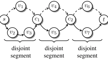
Fig. 4. A link-disjoint path-pair(π1, π2)illustrated in the dashed and solid line. It contains the disjoint segmentss(π1, π2)c1,c1(π1, π2)c2,c2(π1, π2)t, respectively, wherec1andc2are common nodes.
the definedL-LSP problem. Accordingly, in the third stage, we construct the sought pair of paths of a link-disjoint path-pair solution(π1, π2)out of the links of the BF solution. Then, the algorithm outputs the optimal solution(π1, π2).
The following theorem states the correctness of the MWLD-Upper-BCN Algorithm.
Theorem 4.1:Given are a networkG(V, E), a pair of nodess andt, and an upper bound constraint on the number of common nodes k. If there exists a link-disjoint path-pair of at most k common nodes, then the MWLD-Upper-BCN Algorithm returns a feasible weight-shortest link-disjoint path-pair that is a solution to the MWLD-Upper-BCN Problem 2.1; otherwise, the algorithm fails.
In order to establish the proof, we begin by observing that the structure of any link-disjoint path-pair(π1, π2)is composed of node-disjoint subpath-pairs between its common nodes. For a given link-disjoint path-pair(π1, π2), we define the common node set as the ordered set of common nodes along the paths π1 andπ2 including s andt, i.e. {c∈V|c∈π1 and c∈π2}. We note that the common nodes must appear in the same order in the two paths (assuming they are simple). Otherwise, if for instance for two common nodes c1, c2 we have π1 = s c1 c2 t, π2 =s c2 c1 t, they can be replaced by two pathss c1 t, s c2 t, obtained by switching their subpaths while reducing the total weight and the number of common nodes.
Accordingly, we define a disjoint segment ci(π1, π2)ci+1
between two sequential common nodes ci and ci+1 in the common node set as the node-disjoint subpath-pairs ofπ1 and π2 between ci andci+1. The above definitions are illustrated
in Fig. 4.
The weight of a disjoint segment W(ci(π1, π2)ci+1) is de-fined as the sum of all link weights in the disjoint segment, i.e. W(ci(π1, π2)ci+1) = P
e∈ci(π1,π2)ci+1we. Accordingly, a shortest disjoint segment is a disjoint segment ci(π1, π2)ci+1
of minimum weight among all possible disjoint pairs of paths fromci toci+1.
Lemma 4.1:Any optimal solution(π1, π2)to the respective MWLD-Upper-BCN Problem is such that all its disjoint seg-ments are shortest disjoint segseg-ments.
˜
c1 ˜c2 ˜ck ˜ck+1
(a) Subpaths between nodes˜c1and˜ck+1in the auxiliary network
˜
G( ˜V ,E˜)
c1 c2 ck ck+1
a a
[image:6.612.66.282.65.232.2](b) The respective paths nodesc1 and ck+1 in the original networkG(V, E)
Fig. 5. An illustrative graph used in the Proof of Lemma 4.2
c1(π1, π2)c2 between common nodes c1 and c2. Assume by
contradiction that there is a disjoint pair of paths from c1 to c2,c1(cπ1,cπ2)c2, with a lower weight, i.e. W(c1(cπ1,cπ2)c2)<
W(c1(π1, π2)c2). Let us construct a link-disjoint path-pair (cπ1,cπ2) out of the optimal solution (π1, π2) by replacing the
disjoint segment c1(π1, π2)c2 with c1(cπ1,cπ2)c2. Without loss
of generality, assume the links of π1, π2∈c1(π1, π2)c2 are
re-placed withcπ1,πc2∈c1 (cπ1,πc2)c2, respectively. In casecπ1orcπ2
are not simple paths, make them simple by omitting their loops. Note that this loop omission might only improve the number of common nodes along (π1,c cπ2), i.e. C(cπ1,cπ2)≤ C(π1, π2). Moreover,
W(cπ1,cπ2)< W(π1, π2)
which contradicts the assumption that (π1, π2) is the optimal survivable connection of the respective MWLD-Upper-BCN Problem.
Lemma 4.1 justifies the construction in step1of the MWLD-Upper-BCN Algorithm (Fig. 3) in which the links in the auxiliary network G˜( ˜V ,E˜) are associated with the shortest disjoint segments between all pairs of nodes in the network.
We proceed to show that we can obtain a pair of simple paths from any (optimal) solution to the BF algorithm in stage2 of the MWLD-Upper-BCN Algorithm. Consider a link˜ebetween
˜
u and v˜ in the auxiliary network G˜( ˜V ,E˜) which represents the disjoint segment u(π1, π2)v in G. We say that two links ˜
e1 and e˜2 in the auxiliary network G˜( ˜V ,E˜) representing the disjoint segments c1(π1, π2)c2 and c3(π1, π2)c4 are mutually node disjointif their corresponding segments do not have any common nodes (ignoring c1,c2,c3 andc4).
Lemma 4.2:Any optimal solution˜πof theL-LSP problem in stage2of the MWLD-Upper-BCN Algorithm (Fig. 3) is such that all its links are mutually node disjoint.
Proof: Let π˜ be the solution of the L-LSP problem in stage 2. Consider some arbitrary two links in the solution, namely˜c1→c2˜ and˜ck →˜ck+1, which are depicted in Fig. 5a.
These links represent the disjoint segments c1(π
1 1, π
1 2)c2 and ck(π
2 1, π
2
2)ck+1 depicted in Fig. 5b. Assume by contradiction
that they are not mutually node disjoint, i.e. ˜c1 → ˜c2 and
˜
ck → c˜k+1 contain a common node a illustrated, as in Fig. 5b. Without loss of generality, assume that the common node abelongs toπ1
1 andπ21, i.e. the top path in Fig. 5b. Consider the pairs of paths (γ1, γ2) in the original network, where γ1 is composed of path π1
1 till a and path π12 from a (depicted in Fig. 5b by straightly connecting node athrough the dotted arrow) while γ2 is composed from the bottom original paths depicted in Fig. 5b. Evidently, γ1 and γ2 consist of disjoint paths, therefore, there is a link ˜c1 → ˜ck+1 in the auxiliary network illustrated by the dotted link in Fig. 5a. Note the weight of this linkmust be at most the weight of the bottom path between˜c1and˜ck+1depicted in Fig 5a. Accordingly, for the given π, replace the subpath between˜ ˜c1 and ˜ck+1 with the link ˜c1 → c˜k+1, thus creating a new path π. Clearly,ˆ P
˜
e∈πˆw˜˜e<Pe˜∈˜πw˜˜eand the number of links inπˆ is at most
the number inπ. This contradicts the optimality of˜ ˜π. The following two lemmas, namely Lemmas 4.3 and 4.4, prove Theorem 4.1.
Lemma 4.3:If there is no solution to theL-LSP problem in stage 2 of the MWLD-Upper-BCN Algorithm, then there is no solution to the MWLD-Upper-BCN Problem.
Proof:Assume by contradiction that(π1, π2)is a solution to the MWLD-Upper-BCN Problem. Given an upper bound k, (π1, π2)satisfies C(π1, π2)≤k and minimizesW(π1, π2). As previously mentioned, the structure of (π1, π2) contains disjoint segments (Fig. 4). According to Lemma 4.1, the disjoint segments of (π1, π2) are shortest disjoint segments. Hence, consider the pathγthat contains at mostk+ 1links equivalent to the disjoint segments in the auxiliary networkG˜( ˜V ,E˜). The pathγ solves theL-LSP problem in stage 2, which contradicts the assumption that there is no solution to it.
Lemma 4.4: If there is a solution to L-LSP problem in stage 2 of the MWLD-Upper-BCN Algorithm, then stage 3 of the MWLD-Upper-BCN Algorithm returns a solution to the MWLD-Upper-BCN Problem.
Proof: Consider the L-LSP solution γ in the auxiliary networkG˜( ˜V ,E˜), which contains at mostLlinks. At stage 3, we decompose a link-disjoint path pair(π1, π2)from theL-LSP solution γ by transforming each link into a disjoint segment. Lemma 4.2 ensures that the “disjoint links” are mutually node-disjoint, therefore enabling to construct a pair of link-disjoint simple paths with at most k common nodes. Given an upper bound k, (π1, π2) satisfies C(π1, π2) ≤ k and minimizes W(π1, π2), hence it solves the MWLD-Upper-BCN Problem.
We proceed to analyze the running time of the MWLD-Upper-BCN Algorithm. As mentioned, the input size is rep-resented by N and M, which are the numbers of nodes and links in the network, respectively. We denote byBF(|V|,|E|)
andD(|V|,|E|)the running time expressions of the employed (standard) BF algorithm and NDSP algorithm respectively.
Theorem 4.2: The time complexity of the MWLD-Upper-BCN Algorithm isO(N2·D(N, M)+BF(N, N2)), i.e.O(M· N2+N3·log(N)).
construct a new network from the node-disjoint shortest paths between every two nodes. As each original network node is split, the running time of first step of stage 1 isO(N). Next, at the second step of stage 1, we perform the Disjoint Shortest Path algorithm for each pair of nodes in totalN2 times whose running time is O(N2 ·D(N, M)). At stage 2 we run the BF algorithm in the new constructed network, which contains exactly the same number of nodesNand at mostN+N2links, where the complexity of this step isBF(N, N2). At stage 3, we go over all the links in the new network, whose running time is O(N2). Therefore, the total complexity of the MWLD-Upper-BCN Algorithm can be described asO(N+N2·D(N, M) + BF(N, N2) +N2) =O(N2·D(N, M) +BF(N, N2)). Now, we examine the complexity ofD(|V|,|E|)andBF(|V|,|E|). The node-disjoint shortest pair algorithm can be performed in O(|E|+|V| ·log(|V|))[6]. The presented BF Algorithm in 3 can be performed inO(|E| ·L), whereLis the constraint size. Since L is bounded by |V| the algorithm can be executed in a polynomial time ofO(|V| · |E|). Thus, we conclude that the time complexity of MWLD-Upper-BCN algorithm is bounded byO(M ·N2+N3·log(N)).
B. MWLD-Upper-BCN with Selective Common Nodes
From a practical perspective, the common nodes of the de-sired link-disjoint path pair might consist of a special property, e.g. having a retransmission functionality or might be classified as a faulty node. Therefore, it can be required to restrict the common nodes to be selected from a (typically small) subset out of the network nodes. In this section, we explain how to imply such a practically crucial restriction through a network transformation which serves as an input to the MWLD-Upper-BCN Algorithm in Fig. 3.
Given are a network G(V, E), a source s and destination t, and a set of allowable common nodes Vc ( V \ {s, t}.
We aim to find a link-disjoint path pair (π1, π2) such that its common nodes must be allowable common nodes, i.e.
{c|c ∈ π1 ∧c ∈ π2} ⊆ Vc. Note that, according to this
new problem definition, the link-disjoint path pair(π1, π2)also constitutes a node-disjoint path pair in terms of the specific set V \Vc. The proposed reduction is based on a transformation,
named the non-allowable node transformation, that denies every nodev∈V\(Vc∪{s, t})from being a common node. The
transformation is depicted in Fig. 6, where each non-allowable nodevis split into two nodesv1˜ andv2˜ connected by a directed link with weight0. The incoming links to v are connected to the first node˜v1and the outgoing links to the second nodev2.˜
The transformation does not change nodes among the allowable common nodesVc (or the nodess, t).
Lemma 4.5: A common node of a link-disjoint path pair
(π1, π2) must have at least an in-degreeand an out-degree of
2.
Proof:Assume by contradiction that a common nodechas an out-degree of1, thus, π1andπ2must contain the outgoing link of c, contradicting the link-disjointness assumption. The same proof proves the in-degree case.
˜
v1 v˜2 v
˜
w˜e = 0
˜
e
Fig. 6. Non-allowable node transformation, applied for every nodev∈V \
(Vc∪ {s, t}).
Theorem 4.3: Neither the node ˜v1 nor the ˜v2 in the non-allowable node transformation can be a common node in a optimal solution of MWLD-Upper-BCN (Problem 2.1).
Proof:Nodev1˜ has an out-degree of1 while node˜v2 has an in-degree of 1. Due to Lemma 4.5 neither of nodes ˜v1 and
˜
v2 can be a common node.
Note that this reduction allows any of the other nodes, i.e.v∈
Vc, to be selected as a common node. Moreover, the new links
added by the non-allowable node transformation whose weights are set to be 0, do not impact the weight of the link-disjoint path pair(π1, π2)solution. Note that for this specific problem variation the MWLD-Upper-BCN Algorithm described in Fig. 3 can be improved as follows. In Stage 1, an auxiliary graphG˜0= ( ˜V0,E˜0)is constructed from the originalGafter it is applied the
transformation in Fig.6. Note that the node-disjoint path pairs can be computed solely between the set of allowable common nodes and the given source and destination, i.e.v∈Vc∪ {s, t},
resulting inO(|Vc|)2 node-disjoint algorithm calculations. The
weight of a link between two nodesu, v∈Vc∪{s, t}is assigned
in a way similar to the MWLD-Upper-BCN Algorithm (Fig. 3). Given that the number of allowable common nodes is relatively small, i.e. |Vc| << N, the time complexity of the
MWLD-Upper-BCN Algorithm can be improved to O(|Vc|2 ·(M +
Nlog(N))).
In the rest of the paper, we will refer to the MWLD-Upper-BCN algorithm with the non-allowable node transformation as Selective Common Nodes MWLD-Upper-BCN (SCN-Upper-BCN).
C. MWLD Paths Maximizing the Common Nodes
In Section III, we established that the MWLD-Lower-BCN problem is NP-Hard. We proceed to relax the lower bound constraint on the number of common nodes by considering the number of common nodes as a secondary objective. The new variant of the problem is defined as follows.
Problem 4.1: Minimum Weight Link Disjoint Paths with Maximum Common Nodes (MWLD-Max-CN) Problem: Given are a network G(V, E), a source node s ∈ V and a destination nodet∈V. Find a link-disjoint path-pair (π1, π2) fromstotwith a maximum number of common nodes among all the weight-shortest link-disjoint path-pairs.
The MWLD-Max-CN Problem can be solved by employing the MWLD-Upper-BCN Algorithm (Fig. 3), where the common node upper bound constraintkis set to be|V| −2. Since there is no link-disjoint path-pair (π1, π2) with more than |V| −2
0 L1 L2 optimal weight
W(node-disjoint)
W(link-disjoint)
max weight improvement
common nodes upper bound
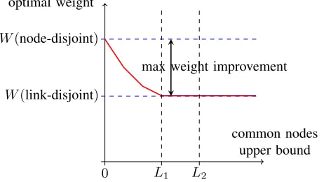
Fig. 7. Spectrum of link-disjoint solutions covered by MWLD-Upper-BCN Algorithm whereL1 and L2 are the minimum and maximum, respectively, number of common nodes in the optimal link disjoint solution.
is achieved by employing theL-Link Bellman-Ford Algorithm in the auxiliary networkG˜( ˜V ,E˜)for L=|V|described in the Appendix. The Bellman-Ford Algorithm is based on a dynamic programming approach, where the distance of each node can be improved by handling all links in the graph iteratively, through arelaxationprocess. The main difference between the Maximum-Link Bellman-Ford Algorithm presented here and the original version is in the relaxation step. Specifically, since in the auxiliary graph we aim at finding a weight-shortest path with maximum number of links, the relaxation is performed also in the case of an equality.
We conclude by describing the space of tractable link-disjoint solutions (depicted in Fig. 7) covered by the solved problems, namely MWLD-Upper-BCN and MWLD-Max-CN. Specifi-cally, the above algorithmic schemes enable the investigation of feasible link-disjoint solutions between the optimal node-disjoint and the optimal link-node-disjoint with maximum number of common nodes. The weight of the solution is expected to be improved by relaxing the constraint in the number of common nodes till the optimal link-disjoint with maximum number of common nodes (i.e., the solution of MWLD-Max-CN). Note that there might be several optimal link-disjoint solutions containing different numbers of common nodes that are covered by the range between L1 and L2 in Fig. 7. A similar behavior is expected to the SCN-Upper-BCN solution, but the link-disjoint solution weight might be higher. In Section VII, we will further analyze the gap in the quality of the solution between the node-disjoint solution and the link-disjoint solution.
V. MWLD PATHS INDIRECTED-ACYCLIC-GRAPH(DAG) TOPOLOGIES
In this section, we consider the three specified problems in Section II, namely MWLD-Upper-BCN, MWLD-Tight-BCN and MWLD-Lower-BCN in the context of DAGs. We present a polynomial-time algorithmic scheme for all problems (includ-ing the MWLD-Tight-BCN and MWLD-Lower-BCN NP-Hard variants).
Input: G˜( ˜V ,E˜)- auxiliary graph with NDSPoP links,s - source,t - destination,w˜e - link weight,
Output:
d[N][N] - link-disjoint path weight with given number of common nodes,π[N][N]- link-disjoint paths.
∀v6=s:d[v][0] = ˜w(s, v)if (s, v)∈E,˜ d[v][0] =∞
otherwise;
d[s][0] = 0; /* initialization */
∀v:π[v][0] =∅; forc= 1 toN−2do
foreach v∈V˜ do
ifu∈V˜|(u, v)∈E˜ existsthen
d[v][c] = min
u∈V˜|(u,v)∈E˜ d[u][c−1] + ˜w(u, v)
π[v][c] =u
else
[image:8.612.50.281.63.193.2]d[v][c] =∞
Fig. 8. Algorithm for MWLD-Upper-BCN, MWLD-Tight-BCN and MWLD-Lower-BCN problems in DAGs
Consider a DAG G(V, E) (satisfying |V| = N), a source node s ∈ V and a destination node t ∈ V such that there is a path between s and t. The algorithm has two stages. First, it constructs an auxiliary graph G˜( ˜V ,E˜) with V˜ = V and links describing possible Node-Disjoint Shortest Pairs of Paths (NDSPoP) in G. This stage is identical to the first stage of the MWLD-Upper-BCN Algorithm (Fig. 3) with the assumption that Gis now a DAG. We refer to the weight of a link (describing the weight of the minimal-weight path pair) between two nodes u, v inG˜ as w˜(u, v). Then, based on the new graph, the second stage of the algorithm calculates for every destination nodet∈V and a given number of common nodesc∈[0, N−2], a link-disjoint path-pair from stotwith exactlyc common nodes of a minimal weight.
For the second stage, described in Fig. 8, we keep two-dimensional arrays d[N][N],π[N][N]. For a node v ∈V˜ and c∈[0, N−2], after thecth iteration, we would like the value of d[v][c] to describe the weight of a link-disjoint path-pair betweenstovinGhaving exactlyccommon nodes. We keep inπ[v][c]the previous common node of path-pair betweensto v withccommon nodes having a minimal weight.
We start by setting d[v][0] = ˜w(s, v) if a link (s, v) exists in G˜ and d[v][0] = ∞ is such a link does not exist. Then, in iteration c ∈ [1, N−2], for each v ∈ V˜ we set d[v][c] = minu∈V|(u,v)∈E˜ d[u][c−1] + ˜w(u, v)
(andd[v][c] =∞if no such link exists). Likewise, we setπ[v][c]to be the nodeu ob-taining this minimum. The algorithm properties are established by the following theorem.
[image:8.612.321.559.136.309.2]weight of a link-disjoint path-pair betweenstov with exactly c common nodes.
Proof: By induction on c. Clearly, with c = 0 common nodes the link-disjoint path-pair is composed of node-disjoint pair of paths that represent a link in G. A path pair with˜ c ≥ 1 common nodes between s and v can be described as a composition of a link-disjoint path pair with c−1 common nodes betweensto some nodeutogether with a node-disjoint pair of path between u to v. Note that in a DAG, unlike a general graph, such composition necessarily results in a link-disjoint path pair betweensandv. The existence of a common link between the two components is impossible as it requires the existence of a cycle. Notice that the maximal number of common nodes cannot be larger thanN−2.
By Theorem 5.1, we can find the solution to each of the problems based on the bound on the number of common nodes. This is done by considering the minimum among the values of d[t][c] for the allowed values of c, i.e. c ∈ [0, k] in the MWLD-Upper-BCN problem,c=kin the MWLD-Tight-BCN problem andc∈[k, N−2]in the MWLD-Lower-BCN problem. The paths can be found by the corresponding values ofπ[t][c], identically to the to the third stage of the MWLD-Upper-BCN Algorithm (Fig. 3).
Time complexity: As stated by Theorem 4.2, we can con-struct the auxiliary graph and calculate its links in O(N+N2·
D(N, M)) =O(N+N2·(M+N ·log(N))). In the second stage, we can consider, up toNtimes, each of theO(N2)links. The total complexity is thusO(M·N2+N3·log(N))).
While the second stage among the two stages in the algorithm described in Fig. 8 has high similarity to the Bellman-Ford algorithm, there are some small but important required changes that eliminate the option to simply apply the known algorithm. First, the calculation of the cost of a shortest path to each node is performed separately (through the use of a two dimensional array) for various numbers of the links inG, illustrating for the˜ selected paths the number of common nodes in G. Similarly, an initial value of a node is not initialized as the corresponding value for the same node in a previous iteration (fewer links) but to infinity, in order to enforce the constraint on the number of links in a path.
VI. MINIMUM-WEIGHTLINK-DISJOINTSECONDPATH In this section, we consider the problem variant of optimizing a second link-disjoint path given one path, where a restriction on their number of common nodes has to be satisfied. We show that an optimal solution of a minimum-weight path is tractable
for all the three constraints of an upper bound, a tight bound or a lower bound on the common nodes number, referred to as Second Path Upper Bound Common Nodes (SP-Upper-BCN), SP-Tight-BCN and SP-Lower-BCN, respectively.
Problem 6.1:Minimum Weight Link Disjoint Second Path with Bounded Common Nodes (SP-Upper/Tight/Lower-BCN) Problem:Given are a networkG(V, E), a source nodes∈V, a destination node t∈V, a first established pathπ1 =s t
Input: G(V, E)- network,s- source,t - destination,we
- link weight,π1=s t- given first path,Γ -allowed values of common nodes number Output:
d[][N][N]- link-disjoint path weight with given number of common nodes,π[][N][N]- link-disjoint paths, π2=s t - optimal second path
V1={v∈π1|v /∈ {s, t}}
E={e= (u, v)∈E|u, v∈V \V1}
d[0][s][0] = 0,d[0][v][0] =∞for v∈V \ {s}
d[0][v][c] =∞for c≥1 and any node v∈V. fori= 1 toN−1 do
foreach v∈V do
forc= 0 toN−2do ifv∈V1,c≥1 then
d[i][v][c] = mind[i−1][v][c],
min(y,v)∈E d[i−1][y][c−1] +w(y, v)
ifv /∈V1 then
d[i][v][c] = mind[i−1][v][c],
min(y,v)∈E d[i−1][y][c] +w(y, v)
[image:9.612.320.560.158.383.2]
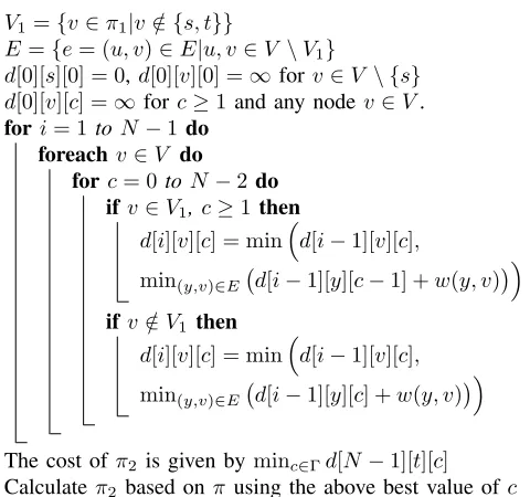
The cost ofπ2 is given byminc∈Γd[N−1][t][c] Calculate π2 based onπ using the above best value ofc Fig. 9. Algorithm for a Minimum-Weight Link-Disjoint Second Path in a general graph
and a set of allowed number of common nodesΓ. Find a link-disjoint pathπ2such that:
min W(π2)
s.t. C(π1, π2)∈Γ.
Let V1 be the nodes in π1 other than the source and destination and let`1 =|V1| be their quantity. The set of the allowed number of common nodes is Γ = {0, . . . , k} in the case of an upper bound, of the form Γ = {k, . . . , `1} in the case of a lower bound or it has a single value Γ = {k} in the case of a tight bound. We solve the problem for a general graph. We look for a single additional path and calculations are performed on the original graphG, as described in Fig. 9.
We maintain 3-dimensional arrays d(for the path cost) and π (for the path nodes). For a node v ∈ V and c ∈ [0, `1], after the ith iteration, we would like the value of d[i][v][c] to
We first eliminate the links ofπ1fromG. For simplicity, we assume that a link weight w(u, v) =∞if there is no link be-tweenutov in the remaining graph and, thus, eliminating any potential selection of the link in a solution. We setd[0][s][0] = 0
and d[0][v][0] =∞ for v∈V \ {s}. Likewise d[0][v][c] =∞
for c≥1 and any nodev∈V. We perform several iterations; to calculate the value d[i][v][c] for a node v ∈ V in iteration i, we distinguish between two cases according to whether v can be counted as a common node (where v ∈ V1) or not (v /∈V1) as follows. (i) v∈V1 - We set d[i][v][c] (for c≥1) as the minimum between its previous value d[i−1][v][c] to
min(y,v)∈E d[i−1][y][c−1] +w(y, v)
. (ii) v /∈ V1 - We setd[i][v][c] (for c≥0) as the minimum between its previous value d[i−1][v][c] to min(y,v)∈E d[i−1][y][c] +w(y, v)
. Respectively, we set π[i][v][c] as its previous value or as the intermediate node y in the link (y, v) achieving the minimal value.
Theorem 6.1:Fori∈[1, N−1], v∈V andc∈[0, N−2], the values of d[i][v][c] are calculated correctly, describing the minimal cost for a paths vof at mostilinks having exactly c common nodes with π1.
Proof: By a simple inductive claim. A path s v of i links withc common nodes can be composed of a paths y of c−1 common nodes, a common node y ∈ V1 and a link y →v. It can also be composed of a paths yof ccommon nodes, a non common node y /∈V1and a link y→v.
In particular, afteri=|V| −1 =N−1iterations, d[i][v][c]
has the weight of a minimal-weight path between sto v that is link-disjoint with π1 and has exactlyc common nodes.
We can derive an optimal conditional second shortest path π2=s t based on the values ofd[N−1][t][c] andπ[N− 1][t][c] according to the restriction on the number of common nodes inΓ. The weight of the conditional second shortest path π2=s tis given byminc∈Γd[N−1][t][c]. The links in the path can be calculated in a reverse order from the values ofπ starting fromπ[N−1][t][c]for the value ofc minimizing the last term.
Time complexity: There are N−1 iterations. In each iter-ation, we consider(N−1) values of the number of common nodes for each of the N nodes, resulting in a complexity of O(N3).
It is easy to see that any first given path followed by a selection of a conditional second path cannot achieve a path pair with a lower weight than that of the optimal path-pair. We recall that such a path-pair can be found for the MWLD-Upper-BCN Problem with an upper bound constraint on the number of common nodes. Furthermore, after a selection of the first path it might be the case that a second link-disjoint path does not exist although a link-disjoint path pair can be found in the graph. We refer to this scenario as blocking. In Section VII we compare the quality of path-pairs found by the two methodologies (for some selection of the first path for the methodology described in this section) and we examine the blocking phenomenon.
VII. SIMULATIONSTUDY
In this section, we demonstrate the advantages of allowing common nodes on the link-disjoint paths on typical network topologies. Accordingly, we examine the gap in the quality of solution between the optimal node-disjoint paths and the op-timal link-disjoint paths by executing the MWLD-Upper-BCN Algorithm described in Section IV-A, and its restriction with an allowed set of common nodes (SCN-Upper-BCN) described in Section IV-B. Furthermore, we analyse the performance of MWLD Second Path algorithms (SP-Upper-BCN, SP-Tight-BCN and SP-Lower-SP-Tight-BCN) introduced in Section VI with a pre-defined weight-shortest first path.
The simulations [25] were performed on a computer run-ning Debian Linux Version 3.3, with four 2.67 GHz Intel Core2 Quad Processors with 12 GB RAM. The networks employed in the simulations are mostly Delaunay-triangulated random planar topologies1 generated with the graph generator
of LEMON [26] with a varying number of nodes, which have enough 4-degree nodes to demonstrate the benefits of our common node approaches, but still resembles the layout of real-world (at least) 2-node-connected networks with a slightly higher average node-degree. We divided the network nodes into two sets: Type A nodes, such as data centers, which are beneficial to have in common in the link-disjoint paths; and Type B nodes which are regular network nodes, such as a client. The links are assumed to be bidirectional having the same weight for both directions. The links weight we is generated
based on the type of its end-nodes, as follows:
• Type A - Type A: uniform random between 1 and 10,
• Type A - Type B: uniform random between 10 and 100,
• Type B - Type B: uniform random between 100 and 1000. Hence, the Type A nodes are connected with high-performance links, while the rest of the network (Type B) nodes linked with low-performance links between themselves and intermediate-performance links to Type A nodes.
For all possible source-destination s−t pairs in the topolo-gies, we calculate the weightWN of the optimal node-disjoint
solution and the weight WL of the optimal link-disjoint
solu-tion. Furthermore, the weight of a link-disjoint solution with a given bound k on the number of common nodes WL,k is
calculated either with MWLD-Upper-BCN, SCN-Upper-BCN or one of the SP-Upper-BCN, SP-Tight-BCN and SP-Lower-BCN algorithms. Specifically, we are interested in the following two performance metrics. First, owing the the highly varying solution costs (because of the wide range of link weight distri-butions) we define therelative improvement as the normalized range between the optimal link-disjoint and optimal node-disjoint solution, i.e., WN−WL,k
WN−WL . Second, we investigate the
percentage (out of all possible source-destination pairs) of our algorithms with a given upper bound k consisting an optimal link-disjoint solution (without any common node restriction), referred to asoptimals−t pairs.
1A maximal planar (i.e., triangulated) graph has3|V| −6links. In contrast,
0.4 0.5 0.6 0.7 0.8 0.9 1
0 1 2 3 4
optimal
s
−
t
pairs
upper boundk 82 links 99 links 137 links
(a) Optimals−tpairs
0.4 0.5 0.6 0.7 0.8 0.9 1
1 2 3 4
relati
v
e
impro
v
ement
upper boundk 82 links 99 links 137 links
[image:11.612.52.297.60.206.2](b) Relative improvement
Fig. 10. MWLD-Upper-BCN performance with 10% of Type A nodes in
N= 50node topologies with varying link number.
A. MWLD-Upper-BCN Algorithm
In this section we analyze the effect of the topology density in random planar networks consisting of50 nodes and either having 137 links (triangulated), or sparser topologies with 99
or 82links with average node-degree of 5.48,3.96, and 3.25, respectively. We evaluate the weight of the disjoint path-pairs among all source-destination pairs using the MWLD-Upper-BCN Algorithm (Fig. 3) with several restrictions on the number of common nodes upper bound, namelyk= 0,1,2,3,4, shown in Fig. 10 with10% (i.e., 5) Type A nodes2.
Fig. 10a depicts the percentage of optimal s −t pairs reachable with the MWLD-Upper-BCN Algorithm. Notably, the optimal link-disjoint path-pair is node-disjoint for more than
45% of the source-destination pairs (k= 0). Furthermore, al-ready with an upper bound ofk= 4on the number of common nodes the optimal link-disjoint path pairs were obtained, i.e., none of the link-disjoint paths contained more than 4 common nodes (except ones−tpair for the 137 link network). It should be noted that, already by allowing a singlek= 1common node, a significant improvement can be reached, specifically, 20%
mores−tpairs can be solved to optimality with our MWLD-Upper-BCN algorithm than with only node-disjoint paths. By allowingk= 2or more common nodes, the weight decrease of the MWLD-Upper-BCN can reach up to 10%−20% relative improvement (Fig. 10b). The improvement is lower in sparser network topologies, as the number of possible detour paths creating opportunities to having nodes in common decreases as well. Hence, the largest benefit of MWLD-Upper-BCN has in the 137link (triangulated) network topology.
B. Selective Common Nodes MWLD-Upper-BCN Algorithm
In the following experiments we check how the restriction on the allowable set of common nodesVcaffects the minimum
weight of the link-disjoint path-pairs. First, we emphasize the
2Intuitively, and also based on our experiments, selecting10%−20%of
the nodes as Type A makes them preferred in the minimum weight link-disjoint path-pairs owing to the link weights. Furthermore, we believe that for applicative scenarios this range could be the most beneficial.
0.75 0.8 0.85 0.9 0.95 1
0 6 12 18 24 30 36 42 48 54
optimal
s
−
t
pairs
allowable common nodes |Vc|
Node-disjoint k= 1
k= 2
k= 3
Fig. 11. Percentage of minimal weight SCN-Upper-BCN solutions with90%
of Type A nodes with different upper boundk on the common nodes in a triangulatedN= 60node,M= 167link network.
difference with the MWLD-Upper-BCN problem, as in the selective common nodes approach the role of the Type A nodes is twofold. On one hand, in MWLD-Upper-BCN the Type A nodes are only encouraged to be common nodes through the randomly generated link weights, but also Type B nodes could be part of a minimum weight MWLD-Upper-BCN solution. However, a minimum weight link-disjoint solution for ans−t pair having a Type B node in common is not part of the design space of the selective common node approach, because the allowable set of common nodesVcis the subset (or all) Type A nodesin SCN-Upper-BCN. Thus, owing to the restriction on the allowed common nodes the weight of the optimal link-disjoint solution might not be achievable for all s−t pairs in some topologies (discussed in Section VII-D).
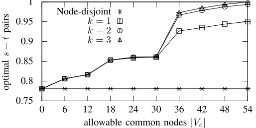
Fig. 11 shows the percentage of optimals−tpairs in a 60 node network (having 56 nodes with degree 4 or larger from which 54 is selected as Type A). First, note that, by increasing the set of allowable common nodes Vc, the percentage of
optimal link-disjoint path-pairs increases, as well. Even by having at most a single node in common in the link-disjoint path-pair (k= 1), the percentage of optimals−t pairs can be improved by about10%. However, further increasingkis only beneficial if the allowable set of common nodes Vc is above 50% of all network nodes.
C. Minimum-Weight Link-Disjoint Second Path Algorithms
In this section, we investigate several real network topologies from Internet Topology Zoo database [27]. Specifically, we remove the 1-degree nodes from the networks to make them 2-node-connected, i.e., a node-disjont path-pair exists between alls−tpairs. However, during our simulations still exhibit the negative effect of the greedy two-step approach, which is often referred to atrap situation. Trap situations occur when a node-disjoint second path could not be found for a fixed first path (e.g., a minimum-weight first path in our simulations), even if the network is 2-node-connected [5].
[image:11.612.310.567.63.192.2]TABLE I
SP-UPPER-BCNALGORITHM RESULTS ON REAL NETWORK TOPOLOGIES FROM THEINTERNETTOPOLOGYZOO[27].
Network topology Blocking ratio (%) Optimals−tpairs (%) Name |V| |E| k= 0 k= 1 k= 2 k=|V| −2
Abilane 11 14 12 12 0 87
Germany 17 25 37 5 2 89
BtEurope 17 30 6 0 0 95
InternetMCI 18 32 11 0 0 92
AS1755 18 33 4 0 0 93
AS3967 21 36 9 1 0 92
BellSouth 21 36 17 9 0 82
BICS 27 42 25 6 3 82
BtNAmerica 36 76 9 1 0 88
0 0.2 0.4 0.6 0.8 1
0 1 2 3 4 5
optimal
s
−
t
pairs
boundk (a) Optimals−tpairs
0.4 0.5 0.6 0.7 0.8 0.9 1
1 2 3 4 5
relati
v
e
impro
v
ement
boundk Lower-BCN
Tight-BCN Upper-BCN
[image:12.612.47.299.93.357.2](b) Relative improvement
Fig. 12. Performance comparison of Lower-BCN, Tight-BCN and SP-Upper-BCN Algorithm with inN= 100nodeM = 287link topology with
10%Type A nodes (legends shown in Fig. 12b refers to both subfigures).
common nodes. The blocking ratios (i.e.,s−t pairs without a solution compared to alls−t pairs) for SP-Upper-BCN with
0%of Type A nodes with increasing kvalue3 are summarized
in Table I (Internet Topology Zoo networks are sparse 2-node-connected topologies with limited 4-degree nodes). Further-more, note that the MWLD-Upper-BCN Algorithm (and SCN-Upper-BCN) always provides a feasible solution in 2-node-connected topologies with an arbitrary k value. In addition, the table indicates the maximum achievable optimals−tpairs with arbitrary many common nodes as well, which is lower than 100% in this scenario, as the greedily selected first (i.e., minimum-weight) path is not always part of a minimum weight link-disjoint path-pair.
Furthermore, we compared the performance of the SP-Lower-BCN and SP-Tight-BCN to the SP-Upper-BCN Algo-rithm in Fig. 12 on a triangulated 100-node planar topology. It should be noted that the blocking ratio of SP-Lower-BCN and SP-Tight-BCN increases to40%askincreases to 5, as the pre-selected fixed first paths with one, two, or more links does not contain so many intermediate nodes that may be common. On the other hand, the SP-Upper-BCN provides a minimum-weight link-disjoint solution to all s−t pairs with k ≥ 1, and only 0.1% of s−t pairs have no solution for k = 0.
3As the links are bidirectional and the topologies are 2-connected, removing
a directed path still leaves a second directeds−tpath in the network. Thus, by increasingkthe number ofs−tpairs without a solution tends to be zero.
0.3 0.4 0.5 0.6 0.7 0.8 0.9 1
0 1 2 3 4 5
optimal
s
−
t
pairs
upper boundk MWLD
SCN SP
(a) Optimals−tpairs
0.5 0.6 0.7 0.8 0.9 1
1 2 3 4 5
relati
v
e
impro
v
ement
upper boundk MWLD
SCN SP
(b) Relative improvement
Fig. 13. Performance comparison of the MWLD-Upper-BCN Algorithm with the selective common nodes (SCN-Upper-BCN) and the minimum-weight link-disjoint second path (SP-Upper-BCN) approach inN = 100nodeM = 287
link topology with10%Type A nodes.
As expected, SP-Tight-BCN has the worst performance in both optimals−tpairs and in relative improvement, as it is part of the design space of the other two approaches. Furthermore, note that the performance of the Upper-BCN problems is always monotonously non-decreasing as k increases because the set of possible solutions always contains the ones with lower k values. However, this is not the case for the Lower-BCN and Tight-BCN problems, thus, they seem to be much limiting and exhibit varying performance by increasingkvalues, depending on the network topology and on the fixed first paths lengths.
D. Comparison of Upper-BCN Algorithms
In Fig. 13 we compare the MWLD-Upper-BCN, SCN-Upper-BCN and SP-Upper-SCN-Upper-BCN approaches proposed for general input graphs in this study. As expected, the MWLD-Upper-BCN Algorithm outperforms of its (restricted) counterpart approaches, which is neither limited by the allowable com-mon nodes set nor by the fixed first path selection. We also emphasize that, owing to these limitations, neither of the two approaches can reach the weight of the optimal link-disjoint solution for alls−tpairs (only up to90%). It is also interesting to observe that, although SP-Upper-BCN provides an optimal solution for less connections than SCN-Upper-BCN, its relative improvement is better fork= 3or more common nodes in the investigated 100nodes Delaunay-triangulated topology.
Furthermore, the SP-Upper-BCN algorithm requires 75 ms on average to calculate a solution for an s−t pair in this network, while the other two algorithms require around 250 ms for all investigated upper bounds. Note that, according to the computational complexity of the methods a significant factor in the running time of the MWLD-Upper-BCN and SCN-Upper-BCN approaches is the construction the auxiliary graph in Stage 1. Once the graph is built, the average running time for ans−tpair drops to 230 ms.
specific algorithms (i.e., SCN-Upper-BCN and SP-Upper-BCN, respectively) can be used to provide minimum-weight link-disjoint paths for these scenarios as well.
VIII. CONCLUSIONS
We studied the problem of finding a minimum weight link-disjoint pair of paths allowing a certain (bounded) number of common nodes. We formalized three variants of the problem, where the number of common nodes satisfies either an upper-bound, a lower-bound or a tight-bound restriction. We estab-lished the NP-Hardness of the lower-bound and the tight-bound problems, while for the upper-bound problem, we proposed a polynomial-time algorithmic solution. Then, we continued to describe how to employ the upper-bound problem solution for solving the problem variant where the common nodes of the link-disjoint pair of paths can be selected only from a (typical small) subset of the network nodes. Moreover, we also described a polynomial-time algorithm for the problem that aims to find a minimum weight link-disjoint pair of paths with a maximum number of common nodes. Under the topological restriction of a DAG, we established an efficient algorithmic scheme for all problem variants (namely, the upper-bound, lower-bound and tight-bound problem). Then, for a given pri-mary path, we established a polynomial algorithmic solution for finding a second minimum weight link-disjoint path for any of the three possible restrictions on the number of common nodes. Finally, through simulations, we analyzed the gap between the optimal node-disjoint and the optimal link-disjoint solutions and we have shown that significant improvement can be reached by allowing the link-disjoint paths having common nodes.
REFERENCES
[1] J. Tapolcai, P.-H. Ho, P. Babarczi, and L. R´onyai, Internet Optical Infrastructure – Issues on Monitoring and Failure Restoration. Springer, 2014.
[2] ITU-T, “G.8032: Ethernet ring protection switching,” 2008.
[3] N. Sprecher and A. Farrel, “MPLS Transport Profile (MPLS-TP) Surviv-ability Framework,” RFC 6372, 2011.
[4] M. Caesar, M. Casado, T. Koponen, J. Rexford, and S. Shenker, “Dynamic route recomputation considered harmful,”Computer Communication Re-view, vol. 40, no. 2, pp. 66–71, 2010.
[5] J. W. Suurballe, “Disjoint paths in a network,”Networks, vol. 4, no. 2, pp. 125–145, 1974.
[6] J. W. Suurballe and R. E. Tarjan, “A quick method for finding shortest pairs of disjoint paths,”Networks, vol. 14, no. 2, pp. 325–336, 1984. [7] K. Menger, “Zur allgemeinen kurventheorie,”Fundamenta Mathematicae,
vol. 10, 1927.
[8] P. Elias, A. Feinstein, and C. Shannon, “A note on the maximum flow through a network,”IRE Trans. on Information Theory, vol. 2, no. 4, pp. 117–119, December 1956.
[9] C. Li, S. McCormick, and D. Simchi-Levi, “The complexity of finding two disjoint paths with min-max objective function,”Discrete Applied Mathematics, vol. 26, no. 1, pp. 105–115, 1990.
[10] D. Xu, Y. Chen, Y. Xiong, C. Qiao, and X. He, “On the complexity of and algorithms for finding the shortest path with a disjoint counterpart,” IEEE/ACM Trans. Netw., vol. 14, no. 1, pp. 147–158, 2006.
[11] A. Orda and A. Sprintson, “Efficient algorithms for computing disjoint QoS paths,” inIEEE INFOCOM, 2004.
[12] L. Guo, K. Liao, H. Shen, and P. Li, “Brief announcement: Efficient approximation algorithms for computing k disjoint restricted shortest paths,” inACM SPAA, 2015.
[13] R. Banner and A. Orda, “The power of tuning: a novel approach for the efficient design of survivable networks,”IEEE/ACM Trans. Netw., vol. 15, no. 4, pp. 737–749, 2007.
[14] J. Yallouz and A. Orda, “Tunable QoS-aware network survivability,” IEEE/ACM Trans. Netw., vol. 25, no. 1, pp. 139–149, 2017.
[15] J. Yallouz, O. Rottenstreich, and A. Orda, “Tunable survivable spanning trees,”IEEE/ACM Trans. Netw., vol. 24, no. 3, pp. 1853–1866, 2016. [16] R. Bhandari, Survivable networks: algorithms for diverse routing.
Springer, 1998.
[17] M. Radetzki, C. Feng, X. Zhao, and A. Jantsch, “Methods for fault tolerance in networks-on-chip,”ACM Comput. Surv., vol. 46, 2013. [18] P. Babarczi, J. Tapolcai, A. Paˇsi´c, L. R´onyai, E. R. B´erczi-Kov´acs, and
M. M´edard, “Diversity coding in two-connected networks,”IEEE/ACM Transactions on Networking, vol. 25, no. 4, pp. 2308–2319, 2017. [19] T. Cormen, C. Leiserson, R. Rivest, and C. Stein, Introduction to
algorithms. MIT press, 2001.
[20] S. Fortune, J. Hopcroft, and J. Wyllie, “The directed subgraph homeo-morphism problem,”Theoretical Computer Science, vol. 10, no. 2, pp. 111 – 121, 1980.
[21] Y. Perl and Y. Shiloach, “Finding two disjoint paths between two pairs of vertices in a graph,”J. ACM, vol. 25, no. 1, pp. 1–9, 1978. [22] Y. Shiloach, “A polynomial solution to the undirected two paths problem,”
J. ACM, vol. 27, no. 3, pp. 445–456, 1980.
[23] T. Tholey, “Solving the 2-disjoint paths problem in nearly linear time,” inSTACS, 2004.
[24] R. Bellman, “On a routing problem,” DTIC Document, Tech. Rep., 1956. [25] “Minimum-Weight Link-Disjoint (MWLD) Paths Simulator, C++ source
code.” [Online]. Available: https://github.com/peterbabarczi/mwldsim [26] “LEMON: A C++ library for efficient modeling and optimization in
networks.” [Online]. Available: http://lemon.cs.elte.hu
[27] S. Knight, H. X. Nguyen, N. Falkner, R. Bowden, and M. Roughan, “The internet topology zoo,”IEEE Journal on Selected Areas in Communica-tions, vol. 29, no. 9, pp. 1765–1775, October 2011.
ACKNOWLEDGEMENTS
APPENDIX
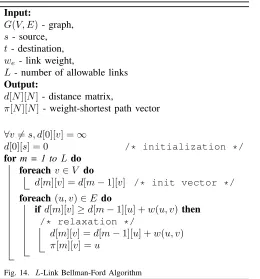
In this Appendix, we present the L-Link Bellman-Ford Al-gorithm, a variant of the well-knownBellman-FordAlgorithm [24], which aims to find a weight-shortest path between two nodes in a weighted directed graph with at most L links. Moreover, in case the weight-shortest path is not unique, the algorithm returns a path with maximum number of links satisfying the upper bound constraint ofL-links. The algorithm is described in Fig. 14 and it is utilized for solving the L-LSP Problem 4.1 and outputs the weight-shortest path with maximum number of links.
Input:
G(V, E)- graph, s - source, t - destination, we - link weight,
L - number of allowable links Output:
d[N][N]- distance matrix,
π[N][N] - weight-shortest path vector
∀v6=s, d[0][v] =∞
d[0][s] = 0 /* initialization */
form = 1 toL do foreach v∈V do
d[m][v] =d[m−1][v] /* init vector */
foreach (u, v)∈E do
if d[m][v]≥d[m−1][u] +w(u, v)then
/* relaxation */
d[m][v] =d[m−1][u] +w(u, v)
[image:14.612.51.311.204.483.2]π[m][v] =u
Fig. 14. L-Link Bellman-Ford Algorithm
The proof of theL-Link Bellman-Ford Algorithm correctness is standard and follows the lines in [19].
Jose Yallouzreceived the B.Sc. and Ph.D. degrees from the Electrical Engineering Department, Tech-nion – Israel Institute of Technology, Haifa, Israel, in 2016 and 2008, respectively. He was a recipient of the Israel Ministry of Science Fellowship in Cyber and advance Computing award. He is mainly interested in computer networks, algorithm design, survivability, SDN and NFV architectures.
Ori Rottenstreich is a researcher in the field of computer networks. In 2015-2017 he was a Postdoc-toral Research Fellow at the department of Computer Science, Princeton university. Earlier, he received the BSc in Computer Engineering (summa cum laude) and PhD degree from the Electrical Engineering department of the Technion, Haifa, Israel in 2008 and 2014, respectively. He was a recipient of the Rothschild Yad-Hanadiv postdoctoral fellowship and the Google Europe PhD Fellowship in Computer Networking. He also received the Best Paper Runner Up Award at the 2013 IEEE Infocom conference as well as the Best Paper Award at the 2017 ACM Symposium on SDN Research (SOSR).
P´eter Babarczi(M’11) received the M.Sc. and Ph.D. (summa cum laude) degrees in computer science from the Budapest University of Technology and Economics (BME), Hungary, in 2008 and 2012, re-spectively. He held appointment as a Post-Doctoral Research Associate with the University of Waterloo, ON, Canada, and the University of Oklahoma, OK, USA. He is an Assistant Professor with the Depart-ment of Telecommunications and Media Informatics at BME and currently also a Post-Doctoral Research Fellow with the Chair of Communication Networks at the Technical University of Munich, Germany. His current research interests include multi-path Internet routing, network coding in transport networks, and combinatorial optimization in softwarized networks. He received the Janos Bolyai Research Scholarship of the Hungarian Academy of Sciences and the Post-Doctoral Research Fellowship of the Alexander von Humboldt Foundation.
Avi Mendelsonis a visiting professor at the CS and EE departments at the Technion and in the EE depart-ment, NTU Singapore. He has a blend of industrial and academic experience in several different areas such as Computer architecture, Power management, security and Real-Time systems. Prof. Mendelson published more than 130 papers in refereed Journals conferences and workshop, and holds more than 25 Patents. Among his industrial roles, he worked for National semiconductors, Intel and Microsoft. Prof. Avi Mendelson is IEEE Fellow, a member of the Board of Governors of the IEEE Computer Society. He is an associate editor of the IEEE trans. on Computers and currently serves as the co-Program-Chair of the ICS-2018 conference that will take place in Beijing, China.