R E S E A R C H
Open Access
Three-dimensional (3D) evaluation of liquid
distribution in shake flask using an optical
fluorescence technique
Amizon Azizan
1,2and Jochen Büchs
2*Abstract
Background:Biotechnological development in shake flask necessitates vital engineering parameters e.g. volumetric power input, mixing time, gas liquid mass transfer coefficient, hydromechanical stress and effective shear rate. Determination and optimization of these parameters through experiments are labor-intensive and time-consuming. Computational Fluid Dynamics (CFD) provides the ability to predict and validate these parameters in bioprocess engineering. This work provides ample experimental data which are easily accessible for future validations to represent the hydrodynamics of the fluid flow in the shake flask.
Results:A non-invasive measuring technique using an optical fluorescence method was developed for shake flasks containing a fluorescent solution with a waterlike viscosity at varying filling volume (VL= 15 to 40 mL) and shaking
frequency (n= 150 to 450 rpm) at a constant shaking diameter (do= 25 mm). The method detected the leading
edge (LB) and tail of the rotating bulk liquid (TB) relative to the direction of the centrifugal acceleration at varying circumferential heights from the base of the shake flask. The determined LB and TB points were translated into three-dimensional (3D) circumferential liquid distribution plots. The maximum liquid height (Hmax) of the bulk
liquid increased with increasing filling volume and shaking frequency of the shaking flask, as expected. The toroidal shapes of LB and TB are clearly asymmetrical and the measured TB differed by the elongation of the liquid particularly towards the torus part of the shake flask.
Conclusion:The 3D liquid distribution data collected at varying filling volume and shaking frequency, comprising of LB and TB values relative to the direction of the centrifugal acceleration are essential for validating future numerical solutions using CFD to predict vital engineering parameters in shake flask.
Keywords:Shake flask, Three dimensional (3D) liquid distribution, Leading edge of bulk liquid (LB), Tail of bulk liquid (TB), CFD, Circumferential liquid distribution, Maximum liquid height
Background
Shake flasks and stirred bioreactors are amongst the popular choice in the development of biotechnological processes. Shake flasks are widely used for biological screenings and process optimizations for the simplicity in geometry, orderly parallel experiments, ease of operation and its low operating cost [1]. In the last years, the main engineering parameters, for instance volumetric power input [2–6], mixing time [7], gas-liquid mass transfer coefficient [8–12], hydromechanical stress [2, 8, 13] and effective shear rate [14] have been
characterized. These vital engineering parameters are significantly governed by the hydrodynamic state in the system in which they influence the yield and quality of the final product in a bioprocess [15].
Computational Fluid Dynamics (CFD) modeling has been used to predict some of the above mentioned en-gineering parameters like volumetric power input and gas-liquid mass transfer coefficient. Zhang et al. [16] and Li et al. [17] simulated two-phase flow fields locating the free interfacial surface area in shake flasks. They predicted the volumetric mass transfer and compared it to the work of Maier and Büchs [9]. It deepens insights about the fluid dynamics within a shake flask. The volume-of-fluid (VOF) method has been applied to solve the continuity equation
* Correspondence:[email protected]
2Aachener Verfahrenstechnik, Biochemical Engineering, RWTH Aachen University, Forckenbeckstrasse 51, 52074 Aachen, Germany
Full list of author information is available at the end of the article
of Navier Stokes [16, 17] for free surface flows which can also be found in other orbitally shaken (microplate or cy-lindrical well) and wave-mixed bioreactor systems [18]. However, in some cases, the models derived may not com-pletely elucidate the real situation in the bioreactors. This might be due to the assumptions of the limited boundary conditions, the applied turbulence models chosen and the spatial and temporal discretization of the transport phe-nomena to a finite-space grid used [15, 18]. Therefore, to answer the numerical uncertainties, CFD models have to be validated or calibrated by measured data.
Many investigations using CFD have been done with stirred bioreactors [15, 18–20] and orbitally shaken bioreac-tors [16, 17, 21–25]. However, to get measured data to val-idate the CFD simulation proves to be a big challenge. In a stirred bioreactor, the interior fluid flow of the bulk liquid is induced by impeller stirring and shows a quite complex pattern. The typical gassed liquid-air dispersions increase the complexity level of fluid flow determination [26]. The details may comprise of the flow of the impeller region, ei-ther simple shear, diverging, converging or rotational vortex flows [27]. Therefore, detailed fluid velocity data from the interior of the bulk liquid in the stirred vessel are needed. For that, a precise and reliable technique is required. The fluid flow data for the bulk liquid can be measured by using contactless and contacting measurement techniques which are e.g. particle image velocimetry [26, 28, 29], laser doppler anemometry [30] and hot film anemometer [31]. In short, the complete 3D characterization of fluid flows in stirred bioreactors requires measurement techniques that are diffi-cult, highly sophisticated and very time-consuming [19].
There were also some attempts to characterize the hydrodynamics of the flow behavior in shake flasks by using particle image velocimetry and laser light tracer methods with different geometries (unbaffled, baffled and coiled) at shaking frequencies of 150 rpm [32], 200 rpm [32] and 80 to 100 rpm [33]. Mixing dynamics in relation to velocity fields and turbulent intensities were reported.
Shake flasks are different from stirred bioreactors. The former develop a specific shape of the rotating bulk liquid inside the bioreactors, resulting from the rotating centrifu-gal field. Thus, this shape of the liquid provides an excel-lent source of information for the validation of CFD simulations. In relation to gas-liquid mass transfer, the hydrodynamics of fluids with waterlike viscosity in shake flask can be described by a ‘two-sub-reactor model’ [10–12], defining mass transfer through the liquid film on the flask wall and base (falling film system) and the bulk li-quid rotating within the flask (mixed stirred tank reactor system). Based on this ‘two-sub-reactor model’ the mass transfer area (a) and the mass transfer coefficient (kL) were modeled and compared with measured values at a broad range of operating conditions. The agreement was found to be quite satisfactory. In stirred bioreactor, the liquid position
with a horizontal surface is well defined, nonetheless, con-taining no information. However, as mentioned above, for shake flasks, it is assumed that the shape and the position of the rotating bulk liquid relative to the centrifugal acceler-ation contain enough informacceler-ation to validate CFD calcula-tions. Therefore, a more complicated measuring approach may not particularly be required.
Previously, the liquid distribution in shake flasks has theoretically been estimated by a simplifying approach disregarding viscosity of the liquid and assuming an ideal frictionless fluid motion [9, 10, 34]. It was reported that the intersection between the rotational paraboloid of the liquid and the inner wall of the shake flasks produces a symmetrical body for the liquid. Validation was under-taken by comparing the computed maximum liquid height to the measured values from photographs [9]. It was also shown that the predicted absolute values of the gas-liquid mass transfer area agree well with those measured by the accelerated sulfite system, if the liquid film formed on the inner glass wall of the flask by the rotating bulk liquid was also taken into account [9]. However, a qualitative com-parison of photographs with simulation results of the sim-plified model of liquid distribution [34], clearly elucidate differences. Whereas the simulated liquid distributions are inherently symmetrical, the real distributions are clearly asymmetrical, showing an extended elongated tail. The same approach was also used in large disposable orbitally shaken cylindrical vessels formulating a well-defined liquid distribution of the bulk liquid, resulting from an inter-section between the rotational liquid paraboloid and the cylindrical bioreactor wall [35].
depth of the rotating bulk liquid perpendicular to the flask wall was not assessed. Doing that would be much more difficult as a usual shake flask is optically not a perfectly symmetrical body and calibration of the liquid depth would be extremely demanding.
Method
Experimental setup of the optical fluorescence measurement technique
A 5 μM fluorescein solution (Fluorescein Acid Yellow 73, Aldrich, Germany) was used as the fluorescent model
solution, buffered with a 100 mM phosphate buffer (Na2HPO4.2H2O ≥ 99%; NaH2PO4.H2O ≥ 98%; Roth, Germany) and adjusted to pH 8 with 5 M sodium hy-droxide (NaOH).
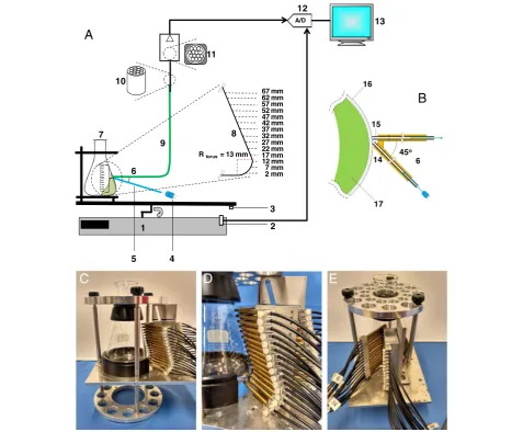
Figure 1a and b show schematic diagrams of the meas-uring setup for the liquid distribution. Fourteen pairs of plastic optical fibers (8: Poly (methyl methacrylate) (PMMA) with cladding material, Conrad Components, Germany) were held in brass holders (14). Two corre-sponding holders were separated by an angle of 45o(6). The pairs were arranged vertically to the side of a 250-mL
9
4
8 7
2 1
R torus = 13 mm
12
13
10
6
67 mm
2 mm 7 mm 12 mm 17 mm22 mm 27 mm 32 mm 37 mm42 mm 47 mm 52 mm 57 mm62 mm
11
3 A/D
5
14 15 16
17 45o
6
C
A
E
B
D
Fig. 1Liquid distribution measurement in shake flasks using an optical fluorescence technique.ashows a schematic diagram of the liquid distribution measurement setup for 250-mL shake flask.bshows a top view of the optical fiber arrangement at the side of the shake flask wall.c,dandeshow a side view, close-up view and 45odistant view of the optical fiber arrangement to the shake flask, respectively. 1) Orbital shaker. 2) Hall sensor. 3)
Magnet for triggering. 4) Light-emitting diode (LED) supplying excitation blue light (465 nm). 5) Optical fiber channeling the excitation blue light to the shake flask. 6) 45oangle distance of the optical fiber arrangement (seen from top view). 7) 250-mL shake flask clamped onto the
shake flask wall (7: Schott Duran, Germany). The height started at 2 mm to 67 mm (with an increment of 5 mm) from the base of the shake flask. Each pair has a 2-mm optical fiber (15) with a core of a 1-mm transparent fiber, one (5) from the light source (light emitting diode) to the shake flask having the fluorescein solution (17) and the other one (9) was from the shake flask to the light receiver (photomultiplier tube) (11).
Blue Indium Gallium Nitride (InGaN) light-emitting diodes (4: Kingbright, Germany) supplied blue excitation light at a peak wavelength of 465 nm. They were alter-nately switched on at different heights. All of the 14 pairs of optical fibers channeling the emission lights from the shake flask were bundled (10) to be in contact to a 15-mm width (11) of the light sensitive area at a photomultiplier tube (Hamamatsu H7827–001, Japan). The blue excitation lights illuminated the fluorescein solution which resulted in emission lights at the peak wavelength of 518 nm. A long pass optical filter (OG 515, Reichmann, Germany) that was positioned prior to the photomultiplier tube, fil-tered the signals received to the wavelength of above 515 nm only. Subsequently, a low noise amplifier and an analog-to-digital converter (A/D) (12) amplified and con-verted the analog signals, using a data acquisition card. The digitized signals were expressed as output voltage (V) and recorded by a computer (13) for further interpretations.
A 250-mL shake flask is comprised of the torus with a radius of 13 mm and the conical upper part. The shapes of the torus and conical parts of the shake flask were calculated accordingly as proposed by [34]. The 250-mL shake flask was pretreated with a boiling 20% nitric acid (HNO3) solution to create hydrophilic conditions at the inner flask wall. The washed and cooled pretreated flask with the attached optical fiber arrangement was then clamped onto the orbital shaker’s table (1: Kuhner, Switzerland) having a hall sensor (2). During a rotation, as the hall sensor was in alignment with a magnet (3) fixed at the shaker’s table, the recording of the signals (output voltage) started. For better viewing of the optical fiber arrangement on the shake flask, Fig. 1c–e show a side view, a close-up photo and a 45o distance view of the measurement setup, respectively.
Using the above described setup, experiments were conducted with varying filling volumes (VL= 15 to 40 mL with an increment of 5 mL) of fluorescein solution at varying shaking frequencies (n = 150 to 450 rpm with an increment of 25 rpm). The shaking diameter was kept constant at 25 mm.
Liquid distribution detection
The measurement setup on the shaker’s table rotated in a clockwise direction (top view). As illustrated in Fig. 2, the uniform rotational motion created centrifugal forces
Tail of bulk liquid (TB)
Magnet for triggering
1 3
2
4 Top view
Orbital shaker
Optical fibers
Centrifugal force
Hall sensor
Optical fibers θθθθ= 0o
90o
180o
270o
-X -Y
+X
+Y Leading edge of
bulk liquid (LB)
origin
A
Fig. 2Shifts of the positions of the rotating bulk liquid in a 250-mL shake flask (40-mm radius) for one complete orbital rotation (illustration is not-to-scale). The start point of a clockwise rotation is at the position 1 when the magnet triggers the hall sensor located at the shaker. Centrifugal forces (red arrows) induced by the orbital rotation exert the bulk liquid towards the wall side of the shake flask along the orbital diameter. The leading edge of a bulk liquid (LB) defines the circulating shift around the shake flask’s circumference having 360ocircular angle. Tail of a bulk liquid (TB) follows
LB circulation in the shake flask. The eye symbol indicates the reference viewing position for the three-dimensional plot as shown in Figs. 4b and 5.adepicts the close-up illustration of the shake flask orientation on angular circular position of liquid detection (θ) [o] and Cartesian
outward along the circumference of the shaking diam-eter orbit on the bulk liquid (not-to-scale drawn dashed red lines). For better interpretation, 90oincremental an-gular positions were set as a basis to the liquid’s location in a shake flask. The location of the set of optical fibers was referred to be at the 0o plane. For a better under-standing of the liquid distribution to be later translated into three-dimensional (3D) plots (see Fig. 4), an eye viewpoint was chosen. The eye viewpoint was positioned to be at the 90oplane as shown in the figure.
The liquid distribution measuring setup recorded the signals every time the liquid moved to the front and passed by the optical fiber’s location. Ten complete rota-tional motions starting from position 1 were recorded to give an average data of liquid distribution in shake flask. The front of the rotating bulk liquid was depicted as the leading edge of the bulk liquid (LB). On the other hand, the end of the bulk liquid was defined as the tail of the bulk liquid (TB). The recorded liquid distribution was a plot of output voltage [V] against the 360o angle of the liquid’s location in the shake flask [o
].
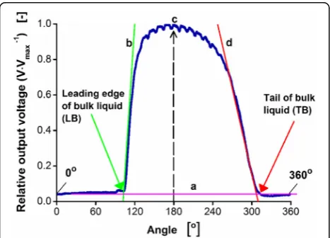
Figure 3 shows an example of a liquid distribution data plot for VL = 25 mL of 5 μM fluorescein solution in a
250-mL shake flask, rotated at n = 200 rpm and
do= 25 mm. It was measured at a height of 22 mm from the base of the shake flask. In this figure, the liquid dis-tribution plot was divided into the following sequence: (starting from the left) the low horizontal line (a: minimal
slope and minimal output voltage), abrupt ascending curve (b: high positive slope with increasing output volt-age), indicating the leading edge (LB) of the bulk liquid, high horizontal curved line (c: minimal slope and maximal output voltage) and the descending curve (d: high to mod-erate negative slope with decreasing output voltage) indi-cating the tail of the bulk liquid (TB). LB and TB angular positions were determined by determining the points of the intersection between (a) and (b) as well as between (a) and (d), respectively. This was done by applying linear re-gression method on the LB and TB regions. The method was justified by a goodness of fit (R2) which was higher than 95%. For instance, in Fig. 3, the determined LB and TB angular positions were identified at 104.84o and 306.85o, respectively.
Result and Discussion
Three-dimensional plot
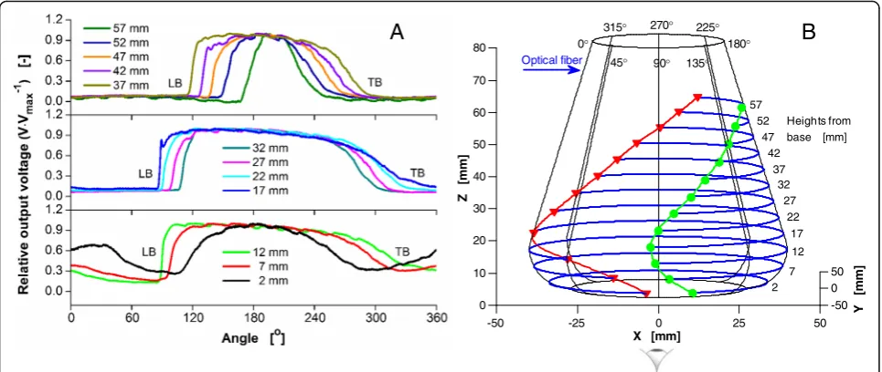
Having all the data collected about the liquid distribu-tion at specific operating condidistribu-tions of the flask, the 3D liquid distribution plots of the bulk liquid on the wall of the shake flask were prepared. Figure 4a shows an ex-ample of the liquid distribution data at the heights of 2 mm to 57 mm from the base of the shake flask with an increment of 5 mm for VL = 40 mL, n = 400 rpm and do= 25 mm. More examples of liquid distribution data are also presented (Additional file 1: Figure S1). The figure depicts the relative output voltage (V/Vmax) value which was defined as the ratio of the measured output voltage to the maximum output voltage detected at each height, versus the 360o circular angle of the shake flask’s circumference. The torus and conical part were referred to as V/Vmax readings at the heights of 2 mm to 12 mm and the heights of above 17 mm, re-spectively. As observed, the width of the rotating bulk li-quid circulating the shake flask became smaller to the higher measurement position at the conical part starting from the height of 17 to 57 mm. From the liquid distri-bution plots (Fig. 4a), LB and TB angular positions were determined according to the method as illustrated in Fig. 3. These angular positions were translated into the corresponding 3D liquid distribution in the shake flask (Fig. 4b). The three-dimensional shape of the shake flask was formed based on 8 vertical planes of 45oangle each. The location of the optical fibers was at the 0oposition. The 3D plot orientation is in accordance to the eye ition viewpoint as shown in Fig. 2. The chosen eye pos-ition allows clearer view of the leading edge (LB) and the tail (TB) of the bulk liquid for the chosen parameters selected. As illustrated in Fig. 4b, the LB was plotted as green solid circle and TB as red solid triangle at each height. The green and red lines connecting the LB and TB angular positions, respectively, represented the circumfer-ential liquid distribution on the shake flask’s wall. The
Fig. 3Example of measured liquid distribution data (360ocircular angle)
plotted as output voltage [V] relative to the maximum values of the output voltage [Vmax] for a 250-mL shake flask rotating at 200 rpm
curve fitting lines were obtained by using a shape preserv-ing interpolation model, specifically the Piecewise Cubic Hermite Interpolating Polynomial (PCHIP) as available in MATLAB.
Figure 4b observes that the exerted rotating bulk liquid concentrated towards the 180o plane in the direction of the centrifugal force. On the other hand, the tail of the bulk liquid was as if dragging behind the leading edge of the bulk liquid. According to the earlier simplifying liquid distribution model [34], the shape of the rotating bulk li-quid should be symmetrical for both the LB and TB. How-ever, the measured liquid distribution data clearly did not reveal a symmetrical LB and TB relative position. Instead, the TB angular positions were elongated to an additional 90ocovering a longer circumferential area. A preliminary comparison of measured data generated in this work and corresponding CFD simulation, originating from the work of Ottow et al. [22] shows a satisfactory agreement (Add-itional file 2 Figure S2). This implies that the depth of the rotating bulk liquid on the flask wall is obviously in reality lower than predicted by the simplifying non-viscosity model [34], what is not an unexpected finding.
Effect of filling volume to maximum liquid height (Hmax), positions of leading edge (LB) and tail of rotating bulk liquid (TB)
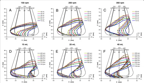
In this investigation, the filling volume was varied while all the other parameters were held constant. Figure 5a–c
depict the compilations of the 3D liquid distribution plots for varying filling volumes (VL= 15 to 40 mL with an increment of 5 mL), at three different shaking fre-quencies (n= 150, 250 and 350 rpm) and at a constant shaking diameter (do= 25 mm).
Figure 5a shows the change of the maximum liquid height (Hmax) (in the z direction) as well as the LB and TB positions with varying VL at n = 150 rpm. At VL of 15 to 40 mL (with an increment of 5 mL), Hmaxvalues are between 25.9 to 33.8 mm from the base of shake flask, respectively. It is obvious that Hmaxincreases as VL increases. It is also observed that the LB positions sequen-tially shift with increasing VLinto the clockwise direction (left), relative to the centrifugal acceleration. On the other hand, despite the increasing VL, TB positions, particularly at the lower torus part, do not differ as much as that seen at the conical upper part of the shake flask.
The above findings are confirmed by Fig. 5b and c with n of 250 and 350 rpm, respectively. The Hmaxfor VL of 15 to 40 mL (with an increment of 5 mL) is re-corded to be from 35.4 mm to 47.0 mm and from 42.0 mm to 56.1 mm, fornof 250 and 350 rpm, respect-ively. Visibly, the rise of Hmaxis influenced relatively to the increasing VL. Additionally, higher VL also shifts the LB and TB positions except for the TB positions at the torus part of the shake flask, as described before. The LB and TB shifts are fairly consistent relative to the increase of VL.
-50 -25 0 25 50
-50 0 50
0 10 20 30 40 50 60 70 80
Y [
m
m
]
180° 225°
135° 90° 270°
X [mm] 45° 315° 0°
Z
[mm]
Optical fiber
2 7
12 17 22 27 32 42 47 52
37 57
Heights from base [mm]
B
A
Fig. 4Measured liquid distribution data (360ocircular angle) for a 250-mL shake flask containing 40 mL of an aqueous 5μM fluorescein solution with 100 mM phosphate buffer (pH 8). Measurement conditions are 400 rpm of shaking frequency and 25 mm of shaking diameter.ashows the output voltage [V] relative to the maximum values of the output voltage [Vmax] detected. The leading edge (LB) and tail of the bulk liquid (TB) are
Effect of shaking frequency to maximum liquid height (Hmax), positions of leading edge (LB) and tail of rotating bulk liquid (TB)
Figure 5d–f show 3D liquid distribution plots of the ro-tating bulk liquid at a fixed do of 25 mm, with varying
n = 150 to 400 rpm and at specific VL of 15, 25 and 40 mL, respectively. Fig. 5d reports on the change of the Hmaxfor a VLof 15 mL at varyingn. Hmaxvalues are be-tween 25.9 and 46.1 mm are recorded for n of 150 to 400 rpm, respectively. It is concluded that Hmaxincreases asnincreases. The LB positions shift sequentially follow-ing the counter clockwise direction (right), relative to the centrifugal acceleration, asnincreases. The phenomena il-lustrates as such that for a constant VL, the bulk liquid is pushed with highern upward and inward, to the conical and torus parts of the shake flask, respectively. In contrast to what is seen for TB positions at constantnand varying VL(see Fig. 5a–c), the TB positions distancing themselves a little apart from each other, particularly at the torus part of the shake flask.
Figure 5e and f with VLof 25 and 40 mL, respectively, confirmed the above assessments. It is clearly seen that as n increases, Hmax also increases. As in Fig. 5e, the Hmax values are between 29.8 mm to 52.0 mm for n of
150 to 400 rpm (with an increment of 50 rpm), respect-ively. Whilst in Fig. 5f, fornof 150 to 400 rpm, the Hmax values are from 33.8 mm to 61.4 mm, respectively.
Conclusion
An extended non-invasive measurement method for asses-sing the liquid distribution in shake flasks by uasses-sing an op-tical fluorescence technique was developed. It consists of 14 sets of optical fibers, 14 light-emitting diodes and one photomultiplier tube, employed for all 14 measurement positions and a fluorescein solution. The 3D circumferen-tial distributions of the rotating bulk liquid were analyzed at varying circumferential heights starting from the base of the shake flask (torus) and extended upward to the conical part. A preliminary comparison of measured data gener-ated in this work and corresponding CFD simulation shows a satisfactory agreement. Leading edge and tail of bulk liquid closely resemble circumferentially in shake flask to the CFD simulation. The information contained in the systematically collected data is very valuable for calibrating and validating Computational Fluid Dynamics (CFD) simulations, to better understand the hydrodynamic flow of fluid in shake flasks. This approach is essential for the numerical determination of some vital engineering
150 rpm 250 rpm 350 rpm
15 mL 25 mL 40 mL
-50 -25 0 25 50
-50 0 50 0 10 20 30 40 50 60 70 80 Y [ m m ] 180° 225° 135° 270° 90°
X [mm]
45°
315°
0°
Z [
m m ] 400 rpm 350 rpm 300 rpm 250 rpm 200 rpm 175 rpm 150 rpm
-50 -25 0 25 50
-50 0 50 0 10 20 30 40 50 60 70 80
Y [
m m ] 180° 225° 135° 270°
X [mm]
90° 45° 315° 0° Z [m m] 400 rpm 350 rpm 325 rpm 300 rpm 250 rpm 200 rpm 175 rpm 150 rpm
-50 -25 0 25 50
-50 0 50 0 10 20 30 40 50 60 70 80 Y [m m ] 180° 225° 135° 270° 90°
X [mm]
45° 315° 0° Z [ m m ] 400 rpm 350 rpm 300 rpm 250 rpm 200 rpm 150 rpm
-50 -25 0 25 50
-50 0 50 0 10 20 30 40 50 60 70 80 Y [m m ] 180° 225° 135° 270° 90°
X [mm]
45° 315° 0° Z [ mm] 40 mL 35 mL 30 mL 25 mL 20 mL 15 mL
-50 -25 0 25 50
-50 0 50 0 10 20 30 40 50 60 70 80 Y [ m m ] 180° 225° 135° 90° 270°
X [mm]
45°
315°
0°
Z [
m m ] 40 mL 35 mL 30 mL 25 mL 20 mL 15 mL
-50 -25 0 25 50
-50 0 50 0 10 20 30 40 50 60 70 80 Y [ m m ] 180° 225° 135° 270° 90°
X [mm]
45°
315°
0°
Z [
m m] 40 mL 35 mL 30 mL 25 mL 20 mL 15 mL
A
B
C
D
E
F
Fig. 5Three-dimensional (3D) illustrations of the bulk liquid position in a 250-mL shake flask containing 5μM fluorescein solution with 100 mM phosphate buffer (pH 8), rotated at 25 mm of shaking diameter, with the same viewing direction as in Figs. 2 and 4. The leading edge (LB) and tail of the bulk liquid (TB) are observed at azimuth and elevation angles of 180oand 6o, respectively.a, bandcindicate 3D illustra-tions of the bulk liquid with varying filling volume and shaking frequency of VL= 15 to 40 mL (at an increment of 5 mL) andn= 150, 250 and
parameters for example volumetric power input, mixing time, gas-liquid mass transfer coefficients, hydromechan-ical stress and effective shear rate in bioprocess develop-ment using shaking flasks. In a succeeding paper, varying liquid distributions CFD calculations utilizing the mea-sured data from this work, initiated at higher viscosities will be reported.
Additional files
Additional file 1: Figure S1.Other examples of the measured liquid distribution data (360ocircular angle) for a 250-mL shake flask containing
25 mL of a 5μM fluorescent solution with 100 mM phosphate buffer (pH 8) at 25 mm shaking diameter.A, B, CandDindicate the liquid distribution measurement conditions of 15 mL and 300 rpm, 20 mL and 200 rpm, 25 mL and 150 rpm, and 30 mL and 350 rpm, respectively. The figures show the output voltage [V] relative to the maximum values of the output voltage [Vmax] detected. The leading edge (LB) and tail of the bulk liquid
(TB) are observed at varying heights starting from 2 mm to 47 mm (with an increment of 5 mm) from the base of the shake flask. The heights of 2 mm to 12 mm refer to the torus of the shake flask while the heights of 17 mm to 47 mm refer to the conical part (as seen in Fig. 4). (PDF 109 kb)
Additional file 2: Figure S2.Computational Fluid Dynamics simulation [22] and three-dimensional (3D) liquid distribution plot from the introduced optical fluorescence technique.Ashows CFD results generated by FLUENT simulations for 25 mL water at 300 rpm shaking frequency, 25 mm shaking diameter in a 250-mL shake flask. Viscosity, density and contact angle used are 0.001003 kg/ms, 998.2 kg/m3and 20o, respectively.Bdepicts the measured 3D liquid distribution in 250-mL shake flask containing an aqueous 5μM fluorescein solution with 100 mM phosphate buffer (pH 8). Data points were collected at varying heights from the base of the shake flask from 2 mm to 42 mm. The black circle and triangle symbols indicate the leading edge of the bulk liquid (LB) and tail of the bulk liquid (TB) for the liquid moving in a clockwise direction. The azimuth and elevation of bothAandBare at 57oand 9.6o, respectively. (PDF 84 kb)
Abbreviations
3D:Three-dimensional; CFD: Computational Fluid Dynamics; do: Shaking
diameter; Hmax: Maximum liquid height; LB: Leading edge of bulk liquid;
M: Molar; mL: Milliliter; mm: Millimeter; mM: Millimolar;n: Shaking frequency; Na2HPO4.2H2O: Disodium hydrogen phosphate dihydrate; NaH2PO4.H2O: Sodium
dihydrogen phosphate monohydrate; nm: Nanometer; rpm: Revolution per minute; TB: Tail of bulk liquid; µM: Micromolar; V: Output voltage; VL: Filling
volume; Vmax: Maximum output voltage
Acknowledgements
The authors wish to thank Udo Kosfeld and Herbert Alt for the electrical and mechanical technical assistances, respectively, as well as to Rahadi Ranom for MATLAB analytics/data mining programming.
Funding
We thank the Malaysia’s Ministry of Higher Learning of Education as scholarship giver to the first author (AA) during the project.
Availability of data and materials
The datasets supporting the conclusions of this article are included within the article.
Author’s contributions
AA made the conceptual design of the liquid distribution measurement device on the shake flask with the assistance of the electrical and
mechanical workshops of the chair, performed the experimental investigations, conducted the result data interpretation, drafted and revised the manuscript. JB initiated the project, financed the resources (AVT), supervised the conceptual design of the liquid distribution measurement, assisted the data interpretation and advised proper corrections of the manuscript. All authors read and approved the final manuscript.
Ethics approval and consent to participate
Not applicable.
Consent for publication
Not applicable.
Competing interests
The authors declare that they have no competing interests.
Publisher’s Note
Springer Nature remains neutral with regard to jurisdictional claims in published maps and institutional affiliations.
Author details
1Faculty of Chemical Engineering, Universiti Teknologi MARA, 40450 Shah Alam, Selangor, Malaysia.2Aachener Verfahrenstechnik, Biochemical Engineering, RWTH Aachen University, Forckenbeckstrasse 51, 52074 Aachen, Germany.
Received: 5 June 2017 Accepted: 18 July 2017
References
1. Büchs J. Introduction to advantages and problems of shaken cultures. Biochem Eng J. 2001;7(2):91–8.
2. Klöckner W, Büchs J. Bioreactor–Design. Shake-Flask Bioreactors. In: Moo-Young M, editor. Comprehensive Biotechnology, Elsevier, vol. 2011. Second ed; 2011. p. 213–26.
3. Büchs J, Maier U, Milbradt C, Zoels B. Power consumption in shaking flasks on rotary shaking machines: I. Power consumption measurement in unbaffled flasks at low liquid viscosity. Biotechnol Bioeng. 2000;68(6):589–93. 4. Büchs J, Maier U, Milbradt C, Zoels B. Power consumption in shaking flasks
on rotary shaking machines: II. Nondimensional description of specific power consumption and flow regimes in unbaffled flasks at elevated liquid viscosity. Biotechnol Bioeng. 2000;68(6):594–601.
5. Büchs J, Zoels B. Evaluation of maximum to specific power consumption ratio in shaking bioreactors. Journal of Chemical Engineering of Japan. 2001;34(5):647–53.
6. Peter CP, Suzuki Y, Rachinskiy K, Lotter S, Büchs J. Volumetric power consumption in baffled shake flasks. Chem Eng Sci. 2006;61(11):3771–9. 7. Tan RK, Eberhard W, Büchs J. Measurement and characterization of mixing
time in shake flasks. Chem Eng Sci. 2011;66(3):440–7.
8. Klöckner W, Büchs J. Advances in shaking technologies. Trends Biotechnol. 2012;30(6):307–14.
9. Maier U, Büchs J. Characterisation of the gas–liquid mass transfer in shaking bioreactors. Biochem Eng J. 2001;7(2):99–106.
10. Maier U, Losen M, Büchs J. Advances in understanding and modeling the gas–liquid mass transfer in shake flasks. Biochem Eng J. 2004;17(3):155–67. 11. Giese H, Azizan A, Kümmel A, Liao A, Peter CP, Fonseca JA, Hermann R,
Duarte TM, Büchs J. Liquid films on shake flask walls explain increasing maximum oxygen transfer capacities with elevating viscosity. Biotechnol Bioeng. 2014;111(2):295–308.
12. Meier K, Klöckner W, Bonhage B, Antonov E, Regestein L, Büchs J. Correlation for the maximum oxygen transfer capacity in shake flasks for a wide range of operating conditions and for different culture media. Biochem Eng J. 2016;109:228–35.
13. Peter CP, Suzuki Y, Büchs J. Hydromechanical stress in shake flasks: correlation for the maximum local energy dissipation rate. Biotechnol Bioeng. 2006;93(6):1164–76.
14. Giese H, Klöckner W, Peña C, Galindo E, Lotter S, Wetzel K, Meissner L, Peter CP, Büchs J. Effective shear rates in shake flasks. Chem Eng Sci. 2014;118:102–13. 15. Sharma C, Malhotra D, Rathore AS. Review of computational fluid dynamics
applications in biotechnology processes. Biotechnol Prog. 2011;27(6):1497–510. 16. Zhang H, Williams-Dalson W, Keshavarz-Moore E, Shamlou PA. Computational-fluid-dynamics (CFD) analysis of mixing and gas–liquid mass transfer in shake flasks. Biotechnol Appl Biochem. 2005;41(1):1–8.
17. Li C, Xia JY, Chu J, Wang YH, Zhuang YP, Zhang SL. CFD analysis of the turbulent flow in baffled shake flasks. Biochem Eng J. 2013;70:140–50. 18. Werner S, Kaiser SC, Kraume M, Eibl D. Computational fluid dynamics as a
19. Hutmacher DW, Singh H. Computational fluid dynamics for improved bioreactor design and 3D culture. Trends Biotechnol. 2008;26(4):66–172. 20. Joshi JB, Nere NK, Rane CV, Murthy BN, Mathpati CS, Patwardhan AW,
Ranade VV. CFD simulation of stirred tanks: Comparison of turbulence models (Part II: Axial flow impellers, multiple impellers and multiphase dispersions). Can J Chem Eng. 2011;89(4):754–816.
21. Weheliye W, Yianneskis M, Ducci A. On the fluid dynamics of shaken bioreactors—flow characterization and transition. AICHE J. 2013;59(1):334–44. 22. Ottow W, Kümmel A, Büchs J. Shaking flask: flow simulation and validation,
VDI Fortschrittsberichte, Conference on Transport Phenomena with Moving Boundaries, 9th-10thOctober, Berlin (Kraume). Germany. 2004;270-279
23. Zhu L-k, B-y S, Wang Z-l, Monteil DT, Shen X, Hacker DL, De Jesus M, Wurm FM. Studies on fluid dynamics of the flow field and gas transfer in orbitally shaken tubes. Biotechnol Progress. 2017;33:192–200.
24. Discacciati M, Hacker D, Quarteroni A, Quinodoz S, Tissot S, Wurm FM. Numerical simulation of orbitally shaken viscous fluids with free surface. Int J Numer Methods Fluids. 2013;71(3):294–315.
25. Tissot S, Reclari M, Quinodoz S, Dreyer M, Monteil DT, Baldi L, Hacker DL, Farhat M, Discacciati M, Quarteroni A, Wurm FM. Hydrodynamic stress in orbitally shaken bioreactors. BMC proceedings. 2011;5(8):39.
26. Hall JF, Barigou M, Simmons MJH, Stitt EH. A PIV study of hydrodynamics in gas–liquid high throughput experimentation (HTE) reactors with eccentric impeller configurations. Chem Eng Sci. 2005;60(22):6403–13.
27. Venkat RV, Stock LR, Chalmers JJ. Study of hydrodynamics in microcarrier culture spinner vessels: a particle tracking velocimetry approach. Biotechnol Bioeng. 1996;49(4):456–66.
28. Wille M, Langer G, Werner U. The influence of macroscopic elongational flow on dispersion processes in agitated tanks. Chemical Engineering & Technology. 2001;24(2):119–27.
29. Willert CE, Gharib M. Digital particle image velocimetry. Exp Fluids. 1991;10(4):181–93.
30. Jaworski Z, Nienow AW, Dyster KN. An LDA study of the turbulent flow field in a baffled vessel agitated by an axial, down-pumping hydrofoil impeller. Can J Chem Eng. 1996;74(1):3–15.
31. Bruun HH. Hot-film anemometry in liquid flows. Meas Sci Technol. 1996;7(10):1301.
32. Mancilla E, Palacios-Morales CA, Córdova-Aguilar MS, Trujillo-Roldán MA, Ascanio G, Zenit R. A hydrodynamic description of the flow behavior in shaken flasks. Biochem Eng J. 2015;99:61–6.
33. Kurata K, Mita H. Qualitative analysis of liquid movement within shake culture flasks using a flow visualization technique.International Symposium on Plant Production in Closed Ecosystem.1996; 440 August: 545–548. 34. Büchs J, Maier U, Lotter S, Peter CP. Calculating liquid distribution in shake
flasks on rotary shakers at waterlike viscosities. Biochem Eng J. 2007;34(3):200–8. 35. Klöckner W, Lattermann C, Pursche F, Büchs J, Werner S, Eibl D. Time efficient
way to calculate oxygen transfer areas and power input in cylindrical disposable shaken bioreactors. Biotechnol Prog. 2014;30(6):1441–56.
• We accept pre-submission inquiries
• Our selector tool helps you to find the most relevant journal • We provide round the clock customer support
• Convenient online submission • Thorough peer review
• Inclusion in PubMed and all major indexing services • Maximum visibility for your research
Submit your manuscript at www.biomedcentral.com/submit