Simulating the mid-Pliocene Warm Period with the CCSM4 model

Geosci. Model Dev., 6, 549–561, 2013 www.geosci-model-dev.net/6/549/2013/ doi:10.5194/gmd-6-549-2013

© Author(s) 2013. CC Attribution 3.0 License.

EGU Journal Logos (RGB)

Advances in

Geosciences

Open Access

Natural Hazards

and Earth System

Sciences

Annales

Geophysicae

Nonlinear Processes

in Geophysics

Atmospheric

Chemistry

and Physics

Atmospheric

Chemistry

and Physics

Atmospheric

Measurement

Techniques

Atmospheric

Measurement

Techniques

Biogeosciences

Open Access Open Access

Biogeosciences

Discussions

Climate

of the Past

Open Access Open Access

Climate

of the Past

Discussions

Earth System

Dynamics

Open Access Open Access

Earth System

Dynamics

Geoscientific

Instrumentation

Methods and

Data Systems

Open Access

_{Geoscientific}

Instrumentation

Methods and

Data Systems

Geoscientific

Model Development

Open Access Open Access

Geoscientific

Model Development

Hydrology and

Earth System

Sciences

Hydrology and

Earth System

Sciences

Ocean Science

Open Access Open Access

Ocean Science

Solid Earth

Open Access Open Access

Solid Earth

The Cryosphere

Open Access Open Access

The Cryosphere

Discussions

Natural Hazards

and Earth System

Sciences

Open Access

Discussions

Simulating the mid-Pliocene Warm Period with the CCSM4 model

N. A. Rosenbloom, B. L. Otto-Bliesner, E. C. Brady, and P. J. Lawrence

National Center for Atmospheric Research, 1850 Table Mesa Drive, Boulder, Colorado, CO 80305, USA

Correspondence to: N. A. Rosenbloom ([email protected])

Received: 27 November 2012 – Published in Geosci. Model Dev. Discuss.: 13 December 2012 Revised: 14 March 2013 – Accepted: 22 March 2013 – Published: 26 April 2013

Abstract. This paper describes the experimental design and model results from a 500 yr fully coupled Commu-nity Climate System, version 4, simulation of the mid-Pliocene Warm Period (mPWP) (ca. 3.3–3.0 Ma). We sim-ulate the mPWP using the “alternate” protocol prescribed by the Pliocene Model Intercomparison Project (PlioMIP) for the AOGCM simulation (Experiment 2). Results from the CCSM4 mPWP simulation show a 1.9◦C increase in global mean annual temperature compared to the 1850 prein-dustrial control, with a polar amplification of∼3 times the global warming. Global precipitation increases slightly by 0.09 mm day−1and the monsoon rainfall is enhanced, partic-ularly in the Northern Hemisphere (NH). Areal sea ice extent decreases in both hemispheres but persists through the sum-mers. The model simulates a relaxation of the zonal sea sur-face temperature (SST) gradient in the tropical Pacific, with the El Ni˜no–Southern Oscillation (Ni˜no3.4)∼20 % weaker than the preindustrial and exhibiting extended periods of qui-escence of up to 150 yr. The maximum Atlantic meridional overturning circulation and northward Atlantic oceanic heat transport are indistinguishable from the control. As com-pared to PRISM3, CCSM4 overestimates Southern Hemi-sphere (SH) sea surface temperatures, but underestimates NH warming, particularly in the North Atlantic, suggesting that an increase in northward ocean heat transport would bring CCSM4 SSTs into better alignment with proxy data.

1 Introduction

This paper describes the experimental design and model re-sults from a 500 yr fully coupled Community Climate Sys-tem, version 4, simulation of the mid-Pliocene Warm Period (mPWP) using the Community Climate System Model, ver-sion 4 (CCSM4). The mPWP (ca. 3.3–3.0 Ma) is the last

period of sustained warmth before the onset of Pleistocene glaciation. Temperature reconstructions from proxies point to a 2–3◦_{C increase in mean global surface temperature over} present day (Dowsett, 2007), with high-latitude temperatu-res as much as 15–20◦C warmer than modern (Ballantyne et al., 2010). The mPWP is also the most recent prolonged period in Earth history when CO2concentrations were sim-ilar to present day. It is, therefore, of particular interest be-cause unlike other warm periods in Earth history, we have relatively abundant proxy data that provide good estimates of both land and ocean temperatures. However, the enigma of the mPWP is that although continental configurations and ocean bathymetry were close to modern and estimated CO2 concentrations (405 ppmv; Pagani, 2010), and were only incrementally higher than present-day values (391 ppm; October 2012, Mauna Loa; http://www.esrl.noaa.gov/gmd/ ccgg/trends/), proxy evidence reveals a much lower pole-to-equator temperature gradient and a more equable seasonal climate overall (Ballantyne et al., 2010). By simulating the mPWP and comparing it to proxy records that show evidence of a strong climate response to CO2forcing, we look through an imperfect lens onto a warm world in hope that it may help us to understand the response of future climate to in-creasingly higher concentrations of atmospheric greenhouse gases. In the process we test the ability of the CCSM4 model to sustain an alternate state of the Earth climate system that looks very different from that of the present day.

2 Model description

2.1 Atmosphere

The atmosphere component model in CCSM4 is the Com-munity Atmosphere Model, version 4 (CAM4) (Neale et al., 2013). The default version of the CAM4 model changed from the spectral core used in CCSM3/CAM3 to the Lin– Rood finite volume (FV) core (Lin, 2004) (CAM4-FV). The CAM4-FV model has improved spatial and temporal aspects of ENSO over the CAM3 model (Richter and Rasch, 2008; Neale et al., 2008; Deser et al., 2012). Changes to cloud frac-tion calculafrac-tions improve Arctic cloud formafrac-tion and lead to a more realistic polar response. However, comparisons with satellite observations indicate that CAM4 continues to have long-standing cloud biases (Kay et al., 2012a), which tend to suppress surface warming and sea ice loss in the Arctic (Kay et al., 2012b). We use a∼1◦horizontal grid for CAM4, with 192×288 latitude/longitude grid cells and a uniform reso-lution of 0.9◦ in latitude×1.25◦ in longitude. CAM4 uses 26 layers in the vertical, which are distributed similarly to CAM3.

2.2 Land

The CCSM4 uses the Community Land Model, version 4 (CLM4, Lawrence et al., 2012). The CLM4 model dif-fers from CLM3, used in CCSM3, by the addition of a carbon–nitrogen (CN) biogeochemical model, revised hy-drology, landcover and land use algorithms, and soil and snow submodels. These modifications lead to improvements in soil water storage, evapotranspiration, surface albedo, and permafrost in fully coupled CCSM4 simulations. The global land precipitation bias is larger in CCSM4 relative to CCSM3, but the global land air temperature bias is re-duced and the annual cycle is improved, especially in high latitudes. CCSM4/CLM4 relies on an embedded river trans-port model (RTM, Branstetter and Famiglietti, 1999) to carry gridcell runoff to the ocean along a model approximation of real-world river networks. The land (CLM4) and atmo-sphere (CAM4) component models share the same 0.9◦ la-titude×1.25◦ longitude horizontal grid; RTM resolution is 0.5◦latitude/longitude grid.

2.3 Ocean

The CCSM4 ocean component model (POP2) is based on the “Parallel Ocean Program”, version 2 (Smith et al., 2010). We use the standard CCSM4 displaced-pole ocean grid with poles in Greenland and Antarctica. The ocean grid has 320× 384 points with nominally 1◦_{resolution except near the} equa-tor, where the latitudinal resolution becomes finer, as de-scribed in Danabasoglu et al. (2006). The number of vertical levels in the ocean increased from 40 to 60 in CCSM4, allow-ing for twenty 10 m levels in the upper ocean. A new over-flow parameterization was added to represent density-driven flows in the Denmark Strait, Faroe Bank Channel, Ross Sea and Weddell Sea (Danabasoglu et al., 2010; Briegleb et al.,

2010). Overall, the CCSM4 ocean model shows clear im-provement in reducing sea surface temperature (SST) and sea surface salinity (SSS) biases relative to the CCSM3 (Gent et al., 2011; Danabasoglu et al., 2012), notably in the North At-lantic, where slight changes in the Gulf Stream and North Atlantic currents reduce but do not eliminate the negative SST and fresh SSS biases along the North Atlantic Cur-rent path, while increasing the warm SST and saline biases off the North American coast. Despite these improvements, the ocean model continues to lose heat content for the dura-tion of the preindustrial control simuladura-tion (Danabasoglu et al., 2012). Maximum North Atlantic overturning (>24 Sv) is stronger in CCSM4 than it was in CCSM3 (>20 Sv) (Gent et al., 2011).

2.4 Sea ice

The CCSM4 sea ice component model (CICE4) is based on version 4 of the Los Alamos National Laboratory “Commu-nity Ice Code” sea ice model (Hunke and Lipscomb, 2008). The sea ice component models in CCSM3 and CCSM4 are generally similar. However, CICE4 incorporates a sophisti-cated new shortwave radiative transfer scheme that signifi-cantly improves the representation of sea ice radiative trans-fer by using inherent optical properties to define scattering and absorption characteristics of snow and ice. The new model also explicitly accounts for melt ponds and the ra-diative impacts of aerosols on sea ice. The rara-diative impact of melt ponds and aerosols on preindustrial Arctic sea ice is 1.1 W m−2annually (Holland et al., 2012), whereas they have negligible impact on Antarctic sea ice. In general, Arc-tic sea ice thickness, areal extent, and spatial pattern com-pare well to observations in the CCSM4 twentieth-century simulations (Jahn et al., 2012). CCSM4 sea ice extents in the Labrador Sea and adjacent North Atlantic have been reduced relative to CCSM3, and the southern Labrador Sea is now ice free. Antarctic sea ice distribution is similar to CCSM3, but still too extensive relative to observations (Landrum et al., 2012). CICE4 uses the same horizontal grid as the ocean component (POP2).

3 Experimental design of mPWP simulation

The PlioMIP models use forcing and boundary condi-tions specified by the USGS Pliocene Research Interpreta-tion and Synoptic Mapping project, version 3 (PRISM3; http: //geology.er.usgs.gov/eespteam/prism/). The PlioMIP proto-col for the AOGCM experiment outlines two model con-figurations: “preferred” and “alternate”, and PRISM3 pro-vides separate boundary condition data packages to accom-modate each configuration. The “preferred” data package includes a land/sea mask that is faithful to what is known about the mPWP, including removal of the West Antarctic Ice Sheet (WAIS). The “alternate” configuration allows mod-eling groups to modify their modern land/sea mask to the ex-tent practical for their model, specifying, for example, West Antarctica as ice-free land. We use the “alternate” configu-ration for the CCSM4 PlioMIP simulation. The forcings and boundary conditions for the mPWP simulation are discussed below and summarized in Table 1.

3.1 CCSM4 preindustrial control simulation

We initialize the mPWP experiment from a long CCSM4 1850 preindustrial (PI) control simulation that was run to ap-proximate equilibrium in accordance with CMIP5 (Coupled Model Intercomparison Project Phase 5) protocols. The PI control simulation uses CLM4 vegetation based on MODIS data (Lawrence and Chase, 2007), topography based on the USGS GTOPO30 digital elevation model, lakes and wetlands derived from Cogley’s (1991) 1◦×1◦dataset for perennial freshwater lakes and swamps/marshes, and glaciers based on the IGBP DISCover dataset (Loveland et al., 2000). Initial conditions for the ocean are described in Gent et al. (2011). The PI control simulated 1300 model yr with constant CO2 (284.7 ppm), N2O (275.68 ppb), and CH4(791.6 ppb), fixed incoming solar radiation at the top of the atmosphere (1360.9 W m−2) and prescribed aerosols (black and organic carbon, sulfate, dust and sea salt). Aerosol concentrations are specified from a historical CCSM chemistry run with pre-scribed emissions (Lamarque et al., 2010), plus a low-level background component to account for volcanic activity (Gent et al., 2011).

3.2 Land/sea mask

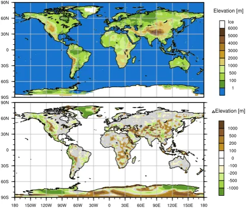
In the mPWP the continents were very close to their current locations, allowing us to use the modern CCSM4 land/sea mask for most of the globe. However, we modify the modern land/sea mask to remove Hudson Bay, a modern epicontinen-tal sea formed by excavation and deformation of the Cana-dian Shield under the weight of Pleistocene ice (Fig. 1), re-quiring the creation of new coupler mapping files. As for our preindustrial control simulation, the Central American Sea-way (Panama GateSea-way) is closed; modern ocean gateSea-ways, including the Bering Strait, Drake Passage, Tasman Gateway, Gibralter Strait, and the Indonesian Gateway, remain open.

Fig. 1. CCSM4 implementation of PRISM3 land ice distribution and elevation map (top) and elevation anomaly (bottom).

3.3 Topography and river routing

We create the mPWP topography by adding the PRISM3 topographic anomaly (mPWP minus modern) (Sohl et al., 2009; Amante and Eakins, 2008) to the CCSM4 modern topography. Implicit in the PRISM3 topographic anomaly is a 25 m increase in mean sea level, which we implement in CCSM4 without changing global coastlines. The largest changes in elevation are over Greenland and West Antarctica, where PRISM3 reduces the volume of continental ice sheets to reflect the 25 m sea level change. Local elevation adjust-ments also affect the North American Rocky Mountains, the Middle East, and Asia. Minor georeferencing discrepancies between the PRISM3 and the CCSM4 base projections are evident in the North American Rocky Mountains and in the Himalayas (Fig. 1). Following PlioMIP protocol (Haywood et al., 2011) we set Hudson Bay and West Antarctica to 25m above sea level. River discharge mapping in the mPWP sim-ulation remains unchanged from present day; drainage across land cells in the emergent Hudson Bay region is routed auto-matically to the nearest ocean grid cell in the Labrador Sea.

3.4 Vegetation

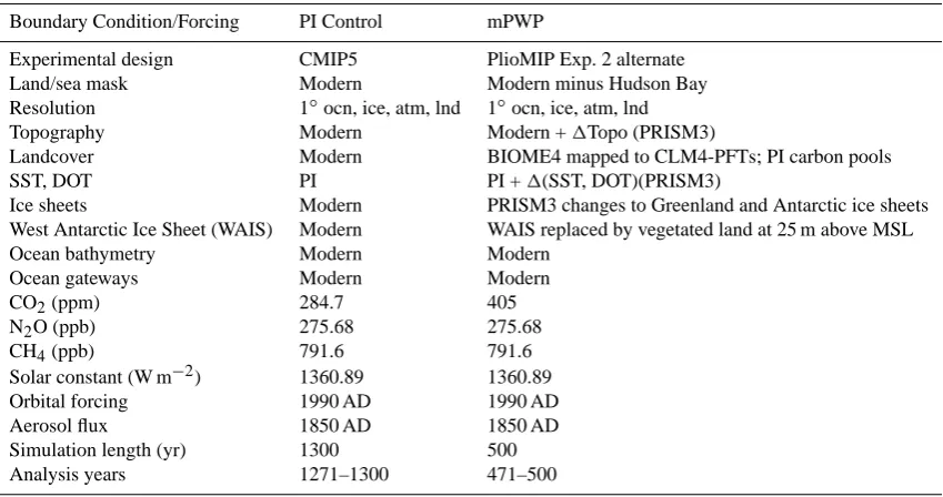
Table 1. Summary of forcings and boundary conditions for the mPWP and 1850 PI control simulations.

Boundary Condition/Forcing PI Control mPWP

Experimental design CMIP5 PlioMIP Exp. 2 alternate

Land/sea mask Modern Modern minus Hudson Bay

Resolution 1◦ocn, ice, atm, lnd 1◦ocn, ice, atm, lnd

Topography Modern Modern +1Topo (PRISM3)

Landcover Modern BIOME4 mapped to CLM4-PFTs; PI carbon pools

SST, DOT PI PI +1(SST, DOT)(PRISM3)

Ice sheets Modern PRISM3 changes to Greenland and Antarctic ice sheets West Antarctic Ice Sheet (WAIS) Modern WAIS replaced by vegetated land at 25 m above MSL

Ocean bathymetry Modern Modern

Ocean gateways Modern Modern

CO2(ppm) 284.7 405

N₂O (ppb) 275.68 275.68

CH4(ppb) 791.6 791.6

Solar constant (W m−2) 1360.89 1360.89

Orbital forcing 1990 AD 1990 AD

Aerosol flux 1850 AD 1850 AD

Simulation length (yr) 1300 500

Analysis years 1271–1300 471–500

biome communities to the modern CLM4/PFT landcover dis-tribution. Using the correlations developed from the mod-ern biome-to-PFT comparison, we spatially extrapolate the CLM4/PFTs to the BIOME4 mPWP biome reconstruction, creating a new mPWP PFT reconstruction for CLM4 that preserves the spatial consistency of modern BIOME4-to-CLM4/PFT biogeography (see Lawrence and Chase (2010) for an analogous application of this approach). This method has the advantage of retaining a physical connection to present-day PFT mapping. Soil type distributions are iden-tical to preindustrial.

3.5 Land ice

The Greenland land ice reconstruction for the mPWP (Hill et al., 2007) greatly reduces the extent of the Greenland Ice Sheet (Fig. 1). In the Southern Hemisphere (SH), PRISM3 reconstructions suggest the WAIS was absent and ice was redistributed over the East Antarctic Ice Sheet (EAIS) rela-tive to present day. Although the “preferred” PlioMIP exper-imental boundary condition removes the WAIS and replaces it with ocean, we use the “alternate” protocol and instead lower the WAIS to 25 m to simulate removal of continental ice. We chose the “alternate” configuration package to avoid extensive modifications to the CCSM4 POP2 ocean grid and bathymetry near the WAIS. We replace land ice with shrubs and arctic grasses over the deglaciated areas of Greenland, WAIS, and EAIS, as prescribed by the BIOME4 plant biome reconstruction (Salzmann et al., 2008).

3.6 Initialization of mPWP simulation

Table 2. Summary of CCSM4 model response.

Variable mPWP Change

from PI

Global surface temperature (◦C) 15.9 1.9 NH surface temperature (20−90◦N) (◦C) 11.1 2.3 SH surface temperature (90−20◦S) (◦C) 8.9 2.2 Global surface temperature over land (◦C) 9.6 2.4 Global precipitation (mm day−1_{) 3.0 0.086} Global precipitation over land (mm day−1) 2.5 0.093 Top of atmosphere energy imbalance (W m−2) 0.02 0.14 Global sea surface salinity (psu) 34.21 –0.14 Global sea surface temperature (◦C) 21.6 1.2 NH Sea ice area (106km2) 9.0 –2.7 (–23 %) SH Sea ice area (106km2) 11.9 –5.1 (–30 %)

Ni˜no 3.4σ(◦C) 0.82 –0.19

4 Results

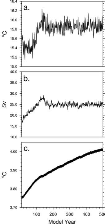
4.1 Approach to equilibrium

Globally averaged mean annual air temperature (Fig. 2a) warms for the first 140 yr of the simulation, then stabiliz-ing, after a small overshoot, by year 180 at 15.9◦C – 1.9◦C warmer than the PI control. The initial ocean response was strongly affected by the warm DOT anomaly applied to the full ocean. The result was a reduction of the Atlantic merid-ional overturning circulation (AMOC), which immediately decreased from an initial strength of 24–17 Sv (Fig. 2b). The overturning circulation recovered within 135 model years, weakly overshooting to a maximum of 28 Sv before stabi-lizing at 26 Sv, similar to the preindustrial CCSM4 AMOC strength. Globally averaged ocean temperature continues to warm by∼0.025◦C per century (Fig. 2c), which is similar in magnitude, although opposite in sign, to the PI control sim-ulation, and indicates that the deep ocean is still coming into equilibrium, a process that takes thousands of years.

4.2 Surface air temperature

Simulated annual and seasonal air temperatures demonstrate warming globally (Fig. 3) relative to the preindustrial control (stippling indicates results are not statistically significant at 95 %). Globally averaged mean annual temperature (MAT) increases by 1.9◦C (Table 2) with enhanced warming over land (2.4◦C) relative to oceans. Zonally averaged MAT in-creases>5◦_{C at high latitudes, while tropical MAT warms} by only∼1◦_{C. Seasonal warming at high latitudes is such} that zonally averaged boreal and austral wintertime tempe-ratures increase by∼6◦C, while summertime temperatures warm by 4−5◦C. High-latitude warming is greater in the Northern Hemisphere (NH).

Fine-scale temperature variability across North America and Asia is caused by differences between the PRISM3 and CCSM4 base projections (Fig. 1). Surface warming over East Antarctic reflects changes to the EAIS topographic profile

Fig. 2. Time series plots of simulated annual mPWP (a) global sur-face air temperature, (b) Atlantic meridional overturning circula-tion, and (c) volume-integrated, global ocean temperature.

(Fig. 1), while warming over Greenland, West Antarctica, and coastal East Antarctica reflects the dual effects of low-ered elevation and landcover conversion from land ice to arctic grasses. The northward expansion of broadleaf and needleleaf trees in BIOME4 and consequent lowering of sur-face albedo contributes to wintertime warming across north-eastern Siberia (Fig. 3). Relative wintertime cooling across southern Siberia (not significant) is similarly related to a con-version from forests to grassland, with a consequent increase in surface albedo. Relative warming and cooling over Hud-son Bay is the result of the land/sea mask conversion from ocean to land.

4.3 Precipitation

Fig. 3. CCSM4 simulated annual and seasonal mPWP surface tem-perature change (◦C) from PI control; stippling indicates results are not statistically significant at 95 % level. Zonally averaged temper-ature change (mPWP minus control) is plotted in the side panels.

pattern of seasonal precipitation indicates a northward shift of the Intertropical Convergence Zone (ITCZ) in response to enhanced NH warming of subtropical SSTs (Fig. 5). Bo-real summer precipitation (June-July-August; JJA) increases by >2 mm day−1 in the eastern equatorial Pacific Basin, the Arabian and Solomon seas, and the monsoon regions of northern Africa and India. JJA precipitation decreases by 1 mm day−1over Siberia and parts of North and South Amer-ica. Precipitation increases significantly in austral summer (December-January-February; DJF) by 1.5 mm day−1 over equatorial Africa, the Bay of Bombay, South China Sea, and Papua New Guinea and the Amazon monsoon region. DJF rainfall decreases by 2–4 mm day−1over the Brazilian High-lands.

Fig. 4. CCSM4 simulated annual and seasonal mPWP precipitation change (mm day−1) from PI control; stippling indicates results are not statistically significant at 95 % level. Zonally averaged precipi-tation change (mPWP minus control) is plotted in the side panels.

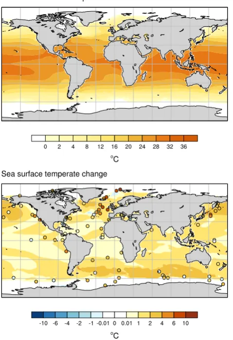
4.4 Sea surface temperature and salinity

Fig. 5. CCSM4 simulated mPWP SST (◦C) (top) and change from PI control (bottom). White regions indicate sea ice in the mPWP simulation (top) and both the mPWP and PI simulations (bottom). Proxy data are plotted as open circles; color code indicates temper-ature change (◦C) from present day.

reconstructed records east of the Kamchatka Peninsula, but falls short of the 4–6◦C of warming indicated further south off the Kuril Islands. CCSM4 SSTs in the North Atlantic warm by 2–4◦C near the southern tip of Greenland, but do not capture the>10◦C of warming suggested by proxy re-constructions. Two limited regions in the North Atlantic cool by 1–2◦C in CCSM4, though not significantly. Proxy recon-structions in the Southern Ocean show regional heterogene-ity with some proxies signaling ∼1◦_{C cooling, and other} areas pointing to as much as 3◦_{C warming. CCSM4} tempe-ratures in the Southern Ocean warm by 2–4◦_{C in the South} Atlantic and Indian Ocean sectors. Simulated temperatures in the South Pacific increase by<2◦C.

Sea surface salinity (Fig. 6) indicates freshening in the polar oceans, where contraction in thickness and extent of sea ice in the mPWP simulation signals an overall reduction in brine rejection, and a consequent fall in sea surface sali-nity relative to preindustrial. A low-salisali-nity plume from the

Fig. 6. CCSM4 simulated sea surface salinity (top) and change from PI control (bottom). White polar regions indicate sea ice in the mPWP simulation (top) and both the mPWP and PI simulations (bottom).

Labrador Sea is carried southward by the Labrador Current, entrained off the coast of Newfoundland and carried east and south along the northern edge of the North Atlantic Drift. Conversely, an increase in the evaporation minus precipi-tation (E-P) in the tropical Atlantic Ocean and midlatitude North Pacific Ocean results in saltier Gulf Stream and East Pacific currents. Increased tropical precipitation and runoff off Southeast Asia lower sea surface salinity from the South China Sea and the Bay of Bengal to the Arafura Sea and the north coast of Australia. Increased runoff from the Pacific Northwest in North America lowers salinity in the Gulf of Alaska.

4.5 Ocean circulation

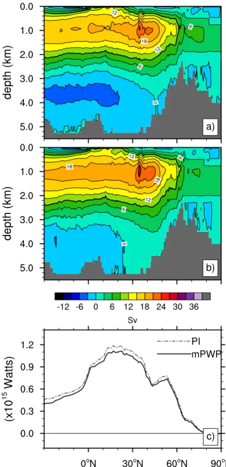
Fig. 7. Eulerian mean meridional overturning circulation (Sv) in the Atlantic Ocean basin for (a) the mPWP, and (b) 1850 PI control; contour interval is 3 Sv. (c) Northward ocean heat transport (×1015 Watts) in the Atlantic Basin for the mPWP (solid) and the PI control (dashed).

in the North Atlantic tracks the northward cycling of warm surface water; counterclockwise flow tracks northward flow-ing deep water from the Southern Ocean. In the mPWP ulation, Southern Ocean water is moving with roughly sim-ilar velocity and strength as in the preindustrial simulation. However, Southern Ocean flow moves much farther north in the mPWP simulation with Antarctic bottom water filling the deep basin up to sill depth.

Northward ocean heat transport in the Atlantic Basin for the simulated mPWP (Fig. 7c) is indistinguishable from preindustrial. This unremarkable response is likely a factor in why the model does not capture the magnitude of warming indicated by North Atlantic temperature proxies. Simulated NH SSTs do not warm enough in the mPWP, particularly in the North Atlantic, whereas SH SSTs are too warm, sug-gesting that enhanced northward ocean heat transport might redistribute enough ocean heat to bring CCSM4 SSTs more in line with proxy evidence.

4.6 Sea ice

The sea ice extent of mPWP (areal %) and thickness (not shown) decrease in both hemispheres (Fig. 8). Overall, sum-mertime sea ice extent is reduced by∼23 % in the Arctic, particularly along the coastal continental shelf, as well as in the Labrador, Greenland and Norwegian seas, where areal extent is reduced by>25 % (Fig. 8). Wintertime sea ice ex-tent (not shown) is reduced by a modest 4 % across the Arc-tic, but drops dramatically in the Pacific Basin, where spa-tial maps indicate a>20 % reduction in the Bering Sea and the Sea of Okhotsk. Similar declines are seen in the Barents Sea, off the southeast coast of Greenland, and in the Labrador Sea along the coast of Newfoundland. Winter and summer-time sea ice thickness (not shown) is reduced by as much as 2 m across the Arctic, with even greater thinning (2–4 m) off the northern coasts of Greenland and the Queen Eliza-beth Islands. Wintertime sea ice thins by up to a meter in the Bering Sea and Sea of Okhotsk, and in the Labrador Sea south to Newfoundland. The PRISM3 sea ice reconstruction (Dowsett, 2007; Robinson et al., 2008; Dowsett and Robin-son, 2009) used by the PlioMIP AGCM Experiment 1 (Hay-wood, 2010) prescribes an ice-free Arctic Ocean during bo-real summer. The CCSM4 simulation of the mPWP shows diminished but persistent seasonal sea ice cover for July-August-September (JAS).

Fig. 8. Spatial maps of CCSM4 simulated Northern Hemisphere (July-August-September; JAS) (top) and Southern Hemisphere (January-February-March; JFM) (bottom) mean sea ice area (%) for the mPWP, the 1850 PI control, and their difference (mPWP minus PI).

4.7 ENSO

The mPWP simulation of Ni˜no3.4 is similar to the preindus-trial control in seasonal cycle and dominant 3–6 yr periodic-ity. However, the Ni˜no3.4, estimated over the last 300 yr of the mPWP, is roughly 20 % weaker (σ =0.82) compared to the PI (σ=1.01), with extended periods of relative quies-cence of up to 150 yr (Fig. 9) compared to similar intervals with only half the duration in the preindustrial. The model does simulate mPWP warming in the eastern equatorial Pa-cific Basin, signaling a relaxation of the zonal SST gradient similar to the response found in the CCSM4 abrupt 4×CO2 simulation (Brady et al., 2013), which also has a weakened Ni˜no3.4 (σ=0.75).

5 Comparison to data

Temperature reconstructions indicate that globally averaged MAT was 2–3◦_{C warmer during the mPWP and as much} as 15–20◦_{C warmer at high latitudes, particularly the} Arc-tic (Ballantyne, 2010). In our CCSM4 mPWP simulation, globally averaged mPWP surface temperatures increase by 1.9◦C relative to preindustrial (Table 2), comparing favor-ably with the reconstructed global average. However, sim-ulated temperatures are conspicuously at odds with proxy records in several critical areas when we plot SST proxy data against corresponding CCSM4 annual SSTs from the near-est latitude/longitude grid cell, and partition the results by

region. Figure 10 shows that, in general, CCSM4 overesti-mates SST warming in the SH extratropics by 1–4◦C. Con-versely, CCSM4 SSTs in the NH extratropics fail to capture the extent of warming expected, particularly in the North At-lantic, where proxy estimates exceed model temperatures by as much as 7◦C. The model shows a uniform SST increase of∼1◦C in the tropics, but does not capture the 2–4◦C of warming indicated by proxy reconstructions. The lack of in-crease in northward ocean heat transport in the Atlantic Basin (Fig. 7) is consistent with the weaker than expected tempera-ture response in the North Atlantic and warmer than expected SSTs in the SH.

6 Relevance to future projections

Fig. 9. The Ni˜no3.4 index (◦C) from the mPWP simulation (top) and the corresponding wavelet power spectrum (bottom).

Fig. 10. PRISM3 reconstructed annual SST plotted against CCSM4 mPWP annual SST for the same latitude/longitude grid cell.

Fig. 11. Zonally averaged MAT anomaly normalized by the global MAT anomaly for the mPWP (solid line), and abrupt 4×CO2 sce-nario simulations with CCSM4 (dashed line).

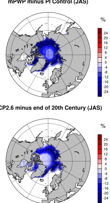
Fig. 12. Spatial maps of the change in NH JAS sea ice area (%) in the mPWP simulation (mPWP minus PI control) (top). Change in NH JAS sea ice area (%) in the IPCC RCP2.6 scenario (RCP2.6, years 2080–2099, minus 20th century, years 1980–1999) (bottom).

We compare mPWP Arctic JAS sea ice concentration against the CCSM4 CMIP5 RCP2.6 simulation (radiative forcing = 2.6 W m−2) in Fig. 12. We show the RCP2.6 en-semble member with the greatest reduction in NH sea ice extent, and compare years 2080–2099 from RCP2.6 against years 1980–1999 from the end of the 20th century simula-tion. JAS arctic sea ice reduction is greater in the mPWP simulation (relative to the PI control), than in the RCP2.6 simulation (relative to the end of the 20th century).

7 Summary

We present results from a 500 yr simulation of the mPWP us-ing the CCSM4 fully coupled model as part of the PlioMIP. The mPWP was the last prolonged period in Earth history when CO2concentrations were similar to present day, result-ing in global mean temperatures that were 2–3◦C warmer than modern and polar temperatures that were as much as 20◦C warmer. The experimental design for the CCSM4 sim-ulation follows the “alternate” PlioMIP protocol for Experi-ment 2. Results from the CCSM4 simulation show a 1.9◦C increase in globally averaged mean annual surface

temper-ature relative to the CCSM4 1850 PI control, with zonally averaged temperature increases of 6◦_{C at high latitudes and} polar amplification of 3 times the global warming. High-latitude warming is greater in the NH than SH. Average sur-face temperature over land increases by 2.4◦C; globally aver-aged sea surface temperature increases by 1.2◦C. Global pre-cipitation increases slightly by 0.09 mm day−1and the ITCZ shifts northward, reflecting greater warming in NH SSTs. Areal sea ice extent decreases in both hemispheres, with a greater decrease in the SH. Arctic sea ice in CCSM4 thins by >2 m, but persists through boreal summer (JAS). The model correctly captures warming in the eastern Pacific Basin, sig-naling a relaxation of the zonal SST gradient, but fails to cap-ture the magnitude of warming in equatorial upwelling areas. Northward ocean heat transport in the Atlantic Basin is in-distinguishable from the control. CCSM4 produces weaker SST warming than reconstructed in the North Atlantic, and greater SST warming than reconstructed in the SH. This bipolar bias suggests an increase in northward oceanic heat transport could bring CCSM4 into better agreement with SST reconstructions.

Acknowledgements. We thank the PRISM group for providing the mPWP datasets for PlioMIP. We also thank the large community of scientists and engineers who contribute to the development of the Community Earth System Model (CESM), including CCSM4. The CESM project is supported by the National Science Foundation and the Department of Energy. The National Center for Atmospheric Research is sponsored by the National Science Foundation, and this work was also supported through grant NSF-EAR-1237211. Computing resources were provided by the Climate Simulation Laboratory (CSL) at NCAR’s Computational and Information Systems Laboratory (CISL), which is sponsored by the National Science Foundation and other agencies. This research was enabled by CISL compute and storage resources. Bluefire, a 4064-processor IBM Power6 resource with a peak of 77 TeraFLOPS provided more than 7.5 million computing hours, the GLADE high-speed disk resources provided 0.4 petabytes of dedicated disk, and CISL’s 12-PB HPSS archive provided over 1 petabyte of storage in support of this research project.

Edited by: D. Lunt

References

Amante, C. and Eakins, B. W.: ETOPO1 1 Arc-Minute Global Re-lief Model: Procedures, Data Sources and Analysis, National Geophysical Data Center, NESDIS, NOAA, U.S. Department of Commerce, Boulder, CO, August 2008.

Bonan, G. B., Levis, S., Kergoat, L., and Oleson, K. W.: Land-scapes as patches of plant functional types: An integrating con-cept for climate and ecosystem models, Global Biogeochem. Cy., 16, 5.1–5.23 doi:10.1029/2000GB001360, 2002.

Brady, E. C., Otto-Bliesner, B. L., Kay, J. E., and Rosenbloom, N. A.: Sensitivity to Glacial Forcing in the CCSM4, J. Cli-mate, 26, 1901–1925, doi:http://dx.doi.org/10.1175/JCLI-D-11-00416.1, 2013.

Branstetter, M. L. and Famiglietti, J. S.: Testing the sensitivity of GCM-simulated runoff to climate model resolution using a par-allel river transport algorithm, Preprints, 14th Conference on Hy-drology, Dallas, TX, USA, American Meteorological Society, 6B.11, 1999.

Briegleb, B. P., Danabasoglu, G., and Large, W. G.: An over-flow parameterization for the ocean component of the Commu-nity Climate SystemModel, NCAR Technical Note NCAR/TN-481+STR, doi:10.5065/D69K4863, 2010.

Cogley, J. G.: GGHYDRO – Global Hydrographic Data Release 2.0, Trent Climate Note 91-1, Dept. Geography, Trent University, Peterborough, Ontario, 1991.

Danabasoglu, G., Large, W. G., Tribbia, J. J., Gent, P. R., Briegleb, B. P., and McWilliams, J. C.: Diurnal coupling in the tropical oceans of CCSM3, J. Climate, 19, 2347–2365, doi:10.1175/JCLI3739.1, 2006.

Danabasoglu, G., Large, W. G., and Briegleb, B. P.: Climate impacts of parameterized Nordic Sea overflows, J. Geophys. Res., 115, C11005, doi:10.1029/2010JC006243, 2010.

Danabasoglu, G., Bates, S. C., Briegleb, B. P., Jayne, S. R., Jochum, M., Large, W. G., Peacock, S., and Yeager, S. G.: The CCSM4 Ocean Component, J. Climate, 25, 1361–1389, doi:10.1175/JCLI-D-11-00091.1, 2012.

Deser, C., Phillips, A. S., Tomas, R. A., Okumura, Y. M., Alexan-der, M. A., Capotondi, A., and Scott, J. D.: ENSO and Pacific Decadal Variability in the Community Climate System Model Version 4, J. Climate, 25, 2622–2651, doi:10.1175/JCLI-D-11-00301.1, 2012.

Dowsett, H. J.: Faunal re-evaluation of Mid-Pliocene conditions in the western equatorial Pacific, Micropaleontology, 53, 447–456, 2007.

Dowsett, H. J. and Robinson, M. M.: Mid-Pliocene equato-rial Pacific sea surface temperature reconstruction: a multi-proxy perspective, Philos. T. R. Soc. A, 367, 109–126, doi:10.1098/rsta.2008.0206, 2009.

Dowsett, H. J., Robinson, M. M., and Foley, K. M.: Pliocene three-dimensional global ocean temperature reconstruction, Clim. Past, 5, 769–783, doi:10.5194/cp-5-769-2009, 2009.

Dowsett, H. J., Robinson, M. M., Stoll, D. K., and Foley, K. M.: Mid-Piacenzian mean annual sea surface temperature analysis for data-model comparisons, Stratigraphy, 7, 189–198, 2010. Gent, P. R., Danabasoglu, G., Donner, L. J., Holland, M. M., Hunke,

E. C., Jayne, S. R., Lawrence, D. M., Neale, R. B., Rasch, P. J., Vertenstein, M., Worley, P. H., Yang, Z.-L., and Zhang, M.: The Community Climate System Model Version 4, J. Climate, 24, 4973–4991, doi:10.1175/2011JCLI4083.1, 2011.

Haywood, A. M., Dowsett, H. J., Otto-Bliesner, B., Chandler, M. A., Dolan, A. M., Hill, D. J., Lunt, D. J., Robinson, M. M., Rosen-bloom, N., Salzmann, U., and Sohl, L. E.: Pliocene Model Inter-comparison Project (PlioMIP): experimental design and bound-ary conditions (Experiment 1), Geosci. Model Dev., 3, 227–242,

doi:10.5194/gmd-3-227-2010, 2010.

Haywood, A. M., Dowsett, H. J., Robinson, M. M., Stoll, D. K., Dolan, A. M., Lunt, D. J., Otto-Bliesner, B., and Chandler, M. A.: Pliocene Model Intercomparison Project (PlioMIP): experi-mental design and boundary conditions (Experiment 2), Geosci. Model Dev., 4, 571–577, doi:10.5194/gmd-4-571-2011, 2011. Hill, D. J., Haywood, A. M., Hindmarsh, R. C. A., and Valdes, P. J.:

Characterising ice sheets during the mid Pliocene: evidence from data and models, in: Deep time perspectives on climate change: Marrying the signal from computer models and biological prox ies, edited by: Williams, M., Haywood, A. M., Gregory, F. J., and Schmidt, D. N., the Micropalaeontological Society, Special Publications, the Geological Society, London, 517–538, 2007. Holland, M. M., Bailey, D. A., Briegleb, B. P., Light, B., and Hunke,

E.: Improved Sea Ice Shortwave Radiation Physics in CCSM4: The Impact of Melt Ponds and Aerosols on Arctic Sea Ice∗, J. Climate, 25, 1413–1430, doi:10.1175/JCLI-D-11-00078.1, 2012. Hunke, E. and Lipscomb, W. H.: CICE: The Los Alamos sea ice model, documentation and software, version 4.0, Los Alamos National Laboratory Tech. Rep. LA-CC-06-012, 76 pp., 2008.

Jahn, A., Bailey, D. A., Bitz, C. M., Holland, M. M., Hunke, E. C., Kay, J. E., Lipscomb, W. H., Maslanik, J. A., Pollak, D., Sterling, K., and Strœve, J.: Late 20th Century Simulation of Arctic Sea Ice and Ocean Properties in the CCSM4, J. Climate, 25, 1431– 1452, doi:10.1175/JCLI-D-11-00201.1, 2012.

Kay, J. E., Hillman, B. R., Klein, S. A., Zhang, Y., Medeiros, B., Pincus, R., Gettelman, A., Eaton, B., Boyle, J., Marchand, R., and Ackerman, T. P.: Exposing Global Cloud Biases in the Com-munity Atmosphere Model (CAM) Using Satellite Observations and Their Corresponding Instrument Simulators, J. Climate, 25, 5190–5207, doi:10.1175/JCLI-D-11-00469.1, 2012a.

Kay, J. E., Holland, M. M., Bitz, C. M., Blanchard-Wrigglesworth, E., Gettelman, A., Conley, A., and Bailey, D.: The Influence of Local Feedbacks and Northward Heat Transport on the Equi-librium Arctic Climate Response to Increased Greenhouse Gas Forcing, J. Climate 25, 5433–5450, doi:10.1175/JCLI-D-11-00622.1, 2012b.

Lamarque, J.-F., Bond, T. C., Eyring, V., Granier, C., Heil, A., Klimont, Z., Lee, D., Liousse, C., Mieville, A., Owen, B., Schultz, M. G., Shindell, D., Smith, S. J., Stehfest, E., Van Aar-denne, J., Cooper, O. R., Kainuma, M., Mahowald, N., Mc-Connell, J. R., Naik, V., Riahi, K., and van Vuuren, D. P.: His-torical (1850–2000) gridded anthropogenic and biomass burning emissions of reactive gases and aerosols: methodology and ap-plication, Atmos. Chem. Phys., 10, 7017–7039, doi:10.5194/acp-10-7017-2010, 2010.

Landrum, L., Holland, M. M., Schneider, D. P., and Hunke, E.: Antarctic Sea Ice Climatology, Variability, and Late Twenti-eth Century Change in CCSM4, J. Climate, 25, 4817–4838, doi:10.1175/JCLI-D-11-00289.1, 2012.

Lawrence, D. M., Oleson, K. W., Flanner, M. G., Fletcher, C. G., Lawrence, P. J., Levis, S., Swenson, S. C., and Bonan, G. B.: The CCSM4 Land Simulation, 1850–2005: Assessment of Sur-face Climate and New Capabilities, J. Climate, 25, 2240–2260, doi:10.1175/JCLI-D-11-00103.1, 2012.

Levitus, S. and Boyer, T. P.: World Ocean Atlas, Volume 4: Temper-ature NOAA Atlas NESDIS 4, U.S. Government Printing Office, 1994.

Lin, S. J.: A “vertically Lagrangian” finite-volume dynamical core for global models, Mon. Weather Rev., 132, 2293–2307, doi:10.1175/1520-0493(2004)132<2293:AVLFDC>2.0.CO;2, 2004.

Loveland, T. R., Reed, B. C., Brown, J. F., Ohlen, D. O., Zhu, Z., Yang, L., and Merchant, J. W.: Development of a global land cover characteristics database and IGBP DISCover from 1km AVHRR data, Int. J. Remote Sens., 21, 1303–1330, 2000. Neale, R. B., Richter, J. H., and Jochum, M.: The impact of

convec-tion on ENSO: From a delayed oscillator to a series of events, J. Climate, 21, 5904–5924, doi:10.1175/2008JCLI2244.1, 2008. Neale, R. B., Richter, J., Park, S., Lauritzen, P. H., Vavrus, S. J., Rasch, P. J., and Zhang, M.: The Mean Climate of the Commu-nity Atmosphere Model (CAM4) in Forced SST and Fully Cou-pled Experiments, J. Climate, online first, doi:10.1175/JCLI-D-12-00236.1, 2013.

Oleson, K. W. and Bonan, G. B.: The effects of remotely-sensed plant functional type and leaf area index on simula-tions of boreal forest surface fluxes by the NCAR land sur-face model, J. Hydrometeorol., 1, 431–446, doi:10.1175/1525-7541(2000)001<0431:TEORSP>2.0.CO;2, 2000.

Pagani, M., Liu, Z., LaRiviere, J., and Ravelo, A. C.: High Earth-system climate sensitivity determined from Pliocene carbon dioxide concentrations, Nat. Geosci., 3, 27–30, doi:10.1038/ngeo724, 2010.

Richter, J. H. and Rasch, P. J.: Effects of convective momen-tum transport on the atmospheric circulation in the Commu-nity Atmosphere Model, version 3, J. Climate, 21, 1487–1499, doi:10.1175/2007JCLI1789.1, 2008.

Robinson, M. M., Dowsett, H. J., Dwyer, G. S., and Lawrence, K. T: Reevaluation of mid-Pliocene North Atlantic sea surface temperatures, Paleoceanography, 23, PA3213, doi:10.1029/2008PA001608, 2008.

Salzmann, U., Haywood, A. M., Lunt, D. J., Valdes, P. J., and Hill, D. J.: A new Global Biome Reconstruction and Data-Model Comparison for the middle Pliocene, Global Ecol. Biogeogr., 17, 432–447, 2008.

Salzmann, U., Haywood, A. M., and Lunt D. J.: The Past is a Guide to the Future? Comparing Middle Pliocene Vegetation With Pre-dicted Biome Distributions for the 21st Century, Philos. T. R. Soc. A, 367, 16 pp. doi:10.1098/rsta.2008.0200, 2009.