Numerical issues associated with compensating and competing processes in climate models: an example from ECHAM-HAM

(1)

Geosci. Model Dev., 6, 861–874, 2013 www.geosci-model-dev.net/6/861/2013/ doi:10.5194/gmd-6-861-2013

EGU Journal Logos (RGB)

Advances in

Geosciences

Open Access

Natural Hazards

and Earth System

Sciences

Open Access

Annales

Geophysicae

Open Access

Nonlinear Processes

in Geophysics

Open Access

Atmospheric

Chemistry

and Physics

Open Access

Atmospheric

Chemistry

and Physics

Open Access Discussions

Atmospheric

Measurement

Techniques

Open Access

Atmospheric

Measurement

Techniques

Biogeosciences

Open Access Open Access

Biogeosciences

Discussions

Climate

of the Past

Climate

of the Past

Discussions

Earth System

Dynamics

Earth System

Dynamics

Discussions

Geoscientific

Instrumentation

Methods and

Data Systems

Open Access

_{Geoscientific}

Instrumentation

Methods and

Data Systems

Geoscientific

Model Development

Geoscientific

Model Development

Discussions

Hydrology and

Earth System

Sciences

Open Access

Hydrology and

Earth System

Sciences

Ocean Science

Discussions

Solid Earth

Discussions

The Cryosphere

Discussions

Natural Hazards

and Earth System

Sciences

Open Access

Discussions

Numerical issues associated with compensating and competing

processes in climate models: an example from ECHAM-HAM

H. Wan1, P. J. Rasch1, K. Zhang1, J. Kazil2,3, and L. R. Leung1 1_{Pacific Northwest National Laboratory, Richland, WA, USA}

2_{Cooperative Institute for Research in Environmental Sciences (CIRES), University of Colorado, Boulder, CO, USA} 3_{NOAA Earth System Research Laboratory (ESRL), Boulder, CO, USA}

Correspondence to: H. Wan ([email protected])

Received: 15 January 2013 – Published in Geosci. Model Dev. Discuss.: 29 January 2013 Revised: 19 April 2013 – Accepted: 10 May 2013 – Published: 26 June 2013

Abstract. The purpose of this paper is to draw attention to the need for appropriate numerical techniques to represent process interactions in climate models. In two versions of the ECHAM-HAM model, different time integration meth-ods are used to solve the sulfuric acid (H2SO4) gas evolution equation, which lead to substantially different results in the H2SO4gas concentration and the aerosol nucleation rate. Us-ing convergence tests and sensitivity simulations performed with various time stepping schemes, it is confirmed that nu-merical errors in the second model version are significantly smaller than those in version one. The use of sequential op-erator splitting in combination with a long time step is iden-tified as the main reason for the large systematic biases in the old model. The remaining errors of nucleation rate in ver-sion two, related to the competition between condensation and nucleation, have a clear impact on the simulated concen-tration of cloud condensation nuclei (CCN) in the lower tro-posphere. These errors can be significantly reduced by em-ploying solvers that handle production, condensation and nu-cleation at the same time. Lessons learned in this work under-line the need for more caution when treating multi-timescale problems involving compensating and competing processes, a common occurrence in current climate models.

1 Introduction

In the past decades, the climate modeling community has been moving gradually towards high-resolution and process-based modeling. More and more complex processes such as the details of aerosol lifecycle and cloud microphysics are

be-ing brought into global and regional climate models. Durbe-ing this evolution, the range of timescales explicitly represented in the models is broadening substantially. From a mathe-matical point of view, this means the system of differential equations is not only expanding but in the meanwhile getting considerably stiffer, posing great challenges to the numerical methods applied in climate models.

Traditionally, numerics is considered by many as the main focus of dynamical core developers and not so much for physicists who design parameterization schemes for sub-grid processes. The air pollution and chemistry transport model-ing community, as well as various numerical weather forecast centers, have paid substantial attention to the use of numer-ical techniques in complex models (e.g., Girard and Delage, 1990; Beljaars, 1991; Teixeira, 2000; Benard et al., 2000; Ja-cobson, 2002; Beljaars et al., 2004; Wood et al., 2007; Za-veri et al., 2008; Schlegel et al., 2012; Tudor, 2012), while climate modelers have focused less on this issue. In this pa-per we present an example from the global aerosol-climate model ECHAM-HAM (Stier et al., 2005; Zhang et al., 2012) to demonstrate that numerical errors associated with stiff sys-tems can lead to significant systematic biases in simulations at typical spatial and temporal scales considered in climate research. The example is also relevant to the numerical treat-ment of many other processes in climate models.

(2)

at most grid points (Zhang et al., 2012). On the one hand, the new scheme outperforms the old one in box model tests presented by Kokkola et al. (2009). On the other hand, com-parisons of the global model simulation with (the still rare) H2SO4 gas measurements seem to suggest that the new model version is associated with larger positive biases (D. O’Donnell, personal communication, 2012). In this paper we carry out convergence tests for the two time stepping schemes and analyze the characteristics of the numerical er-rors. The aim is to identify a better scheme from a numeri-cal perspective, and quantify the remaining biases. Impact of these biases on the simulated aerosol and cloud condensation nuclei (CCN) number concentration is also discussed.

As is elaborated later in the paper, the key to an accu-rate numerical solution of the H2SO4 gas equation is the proper balances between strongly compensating and compet-ing processes. Such situations of process interaction are often encountered in other components of the climate models as well. Examples include the liquid water budget in cloud mi-crophysics (P. Caldwell, personal communication, 2013) and the wind profile in the near-surface levels (Beljaars, 1991). In this paper we consider the sulfuric acid gas equation as a pro-totype problem of this kind. By testing several time stepping methods in addition to those used in HAM1 and HAM2, we attempt to obtain some generally useful conclusions regard-ing the numerical representation of process interactions in climate models.

The remainder of the paper is organized as follows: Sect. 2 introduces the sulfuric acid gas equation in ECHAM-HAM and outlines the time stepping methods. Section 3 presents results of the convergence test and establishes the reference solution. Section 4 focuses on the issue of strongly compen-sating processes, and Sect. 5 the competing processes. Con-clusions from this study are summarized in Sect. 6.

2 Methodology

This section first briefly introduces the ECHAM-HAM model to set the context. The sulfuric acid gas equation is then described, together with the time stepping schemes used in HAM1 and HAM2. Other integration schemes used in the sensitivity experiments are also introduced. Thereafter, the simulations for testing these schemes are described.

2.1 Overview of ECHAM-HAM

ECHAM-HAM is a global aerosol-climate model developed for understanding the distribution, properties and lifecycle of tropospheric aerosols as well as their interactions with cli-mate.

The atmospheric general circulation model ECHAM5 (Roeckner et al., 2003, 2006) solves the hydrostatic equa-tions of fluid motion using the spectral transform method with triangular truncation. In the vertical, the model

uses a pressure-based terrain-following coordinate with discretization methods following Simmons and Burridge (1981). The highest computational level is located at 10 hPa. The large-scale transport of water substances and other trac-ers is handled by the flux-form finite volume algorithm of Lin and Rood (1996), assuming the fields vary with parabolic sub-grid distributions. Cumulus convection and convective tracer transport are described by the mass flux scheme of Tiedtke (1989), with further modifications by Nordeng (1994). The turbulent transport of momentum, heat, mois-ture and tracers is represented by the eddy-diffusivity scheme of Brinkop and Roeckner (1995) which involves a prognos-tic equation for the turbulent kineprognos-tic energy. Short-wave and long-wave radiative transfer calculations follow the methods of Fouquart and Bonnel (1980) and Mlawer et al. (1997), re-spectively.

The aerosol module HAM was first developed by Stier et al. (2005), and has gone through various updates in re-cent years. A summary can be found in Zhang et al. (2012). The aerosol population in the atmosphere is described by the mass concentrations of different chemical species (sulfate, black carbon, organic matter, sea salt, and mineral dust), and the number concentrations of different particle size classes. The particle size distribution is mathematically described by 7 log-normal modes, 4 of which correspond to solu-ble aerosols that are internally mixed (meaning one particle can contain more than one chemical composition), while the other 3 modes are insoluble, and externally mixed (i.e., each particle contains only one chemical species). In the model, aerosols can form in the atmosphere through nucleation pro-cesses. The mechanisms considered in HAM2 include neu-tral and charged nucleation of H2SO4and H2O (Kazil and Lovejoy, 2007; Kazil et al., 2010). In the planetary bound-ary layer over forested areas, the nucleation of H2SO4 and an organic compound can be simulated by the kinetic nu-cleation parameterization of Laakso et al. (2004) and Kuang et al. (2008), or the cluster activation scheme of Kulmala et al. (2006) and Riipinen et al. (2007). Aerosol particles can also be directly released into the atmosphere through natural and/or anthropogenic emission. The emission fluxes are in-teractively calculated for sea salt and dust (Monahan et al., 1986; Smith and Harrison, 1998; Tegen et al., 2002; Cheng et al., 2008), and prescribed for the other species. Micro-physical processes, such as coagulation and condensation of H2SO4 gas, are considered following Vignati et al. (2004). The parameterization of aerosol water uptake is based on the work of Petters and Kreidenweis (2007). Aerosols are re-moved from the atmosphere by gravitational settlement (Stier et al., 2005), turbulent dry deposition (Kerkweg et al., 2006), as well as in-cloud and below-cloud scavenging (Stier et al., 2005; Zhang et al., 2012, and references therein).

(3)

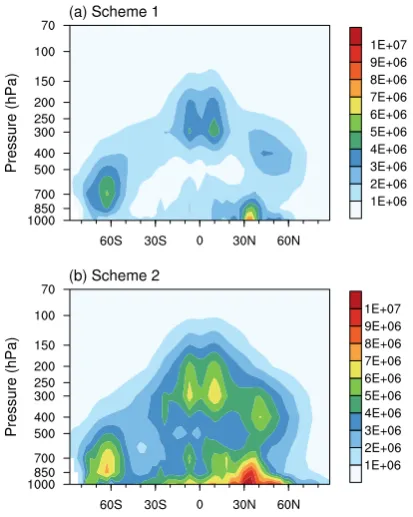
Fig. 1. Annually and zonally averaged sulfuric acid gas concentra-tions (unit: number of molecules per cm3) simulated by two con-figurations of the aerosol-climate model ECHAM-HAM, version 2. Panel (a) corresponds to time stepping scheme 1 in Table 1 which solves the sulfuric acid equation (Eq. 1) using the Euler forward scheme with sequential splitting; Panel (b) uses scheme 2 in Ta-ble 1, originally introduced by Kokkola et al. (2009). The simulation setups are described in Sect. 2.3.

the large-scale and sub-grid-scale transport of aerosols and their precursors. Aerosols affect atmospheric circulation by changing the radiation budget and through their impacts on cloud microphysics (Lohmann et al., 2007; Lohmann and Hoose, 2009).

2.2 Sulfuric acid gas equation

In ECHAM-HAM, an ordinary differential equation (ODE) of the form

dS

dt =P−C·S−N (S) (1)

is included to represent the link between sulfur chemistry and aerosol microphysics. HereS denotes the concentration of H2SO4gas in the unit of molecules per cubic centimeter.P is the source term related to chemical production and trans-port processes.C·Sdescribes the condensation of H2SO4gas on pre-existing aerosol particles.N (S) denotes the H2SO4 gas loss rate due to aerosol nucleation, generally a nonlinear function ofS. Within each step of the time integration, the source termP and the condensation coefficient C are kept constant.

In the old model HAM1, Eq. (1) is solved by the Euler forward scheme using sequential splitting. The concentration Sis updated in three consecutive steps, each considering one term on the r.h.s. of Eq. (1):

S∗=St+1t P (2)

S∗∗=S∗−_{min [}1t C S∗,0.95S∗] (3) St+1t=S∗∗−min [1t N (S∗∗), S∗∗]. (4) Note that in Eq. (3) the H2SO4gas condensation is limited to 95 % of the available amount, while in Eq. (4) there is a lim-iter applied to nucleation to avoid negative concentrations. This algorithm is referred to as “scheme 1” in the remainder of the paper.

In HAM2, a two-step time integration scheme proposed by Kokkola et al. (2009) is employed. First, production and condensation are considered together using

S∗=

St− P

C

e−C1t+P

C. (5)

This expression is an analytical solution of the production-condensation equation (i.e., Eq. 1 withN (S)=0) when as-suming the production rate P and condensation coefficient C are constant within the time interval 1t. Subsequently, the nucleation sink N is computed using the intermediate concentrationS∗, and adjusted with an Euler-backward fac-tor 1/(1+C1t ). (This adjustment factor comes from an at-tempt to discretize Eq. (1) with the Euler-backward scheme in which iterative evaluations of aerosol nucleation are em-ployed to avoid a nonlinear solver. A detailed explanation can be found in Sect. 3 of Kokkola et al. (2009).) The new concentrationSt+1t is given by

St+1t=S∗−min

1t N (S∗) 1+C1t, S∗

. (6)

This integration method is referred to as “scheme 2” in the following. As can be seen in Fig. 1, the use of Eqs. (5) and (6) instead of the old scheme results in considerably higher H2SO4 gas concentrations at most grid points in the model domain. (Details of the simulation setup are given in the next subsection.)

In order to explain this difference and to analyze the properties of the two schemes, the following time stepping schemes are also tested:

– Scheme 1EP: Similar to scheme 1 but using parallel splitting for production and condensation, i.e.,

(4)

and (8) also include the same limiters as in scheme 1 (Eqs. 2–4), for the purpose of a clean comparison be-tween the sequential and parallel splitting of production and condensation.

– Scheme 1Im: Similar to scheme 1EP but replace Eq. (7) by the trapezoidal implicit scheme

S∗=St+1t P−0.51t C (St+S∗) . (9) A limiterS∗=max(0, S∗)is applied, assuming that all available H2SO4 gas, rather than 95 % of it, can con-dense on existing aerosol particles. As discussed later in the last paragraph of Sect. 4.2, this change in the lim-iter helps to eliminate positive errors in regions of high aerosol loading.

– Scheme 2C: Similar to scheme 2 but without the Euler backward adjustment for nucleation, i.e., replace Eq. (6) by (8).

– Scheme 2CP: Use analytical solution for the production-condensation equation as in schemes 2 and 2C (Eq. 5), but parallel splitting between produc-tion/condensation and nucleation, i.e., Eq. (5) followed by

St+1t=max [ 0, S∗−1t N (St)]. (10) The time integration methods described above, except for scheme 2CP, are based on sequential splitting between nucle-ation and the rest of the ODE, limiting the numerical conver-gence to first order. In addition to these schemes, we evaluate two methods that solve production, condensation and nucle-ation simultaneously. These schemes are based on a Taylor expansion of the nucleation sink

N (S)=N (St)+ _d

N dS

t

(S−St)+ · · ·. (11) Substituting Eq. (11) into (1), we get a linearized differential equation

dS

dt = ˆP− ˆC·S (12)

with ˆ

P =P−N (St)+ _d_N

dS

t

St and (13)

ˆ C=C+

_d N dS

t

. (14)

Now that Eq. (12) has constant coefficients within one time step, we can apply the analytical solution to get

St+1t= St− ˆ P ˆ C

!

e− ˆC1t+ ˆ P ˆ

C . (15)

The derivation of Eq. (12) can be interpreted as linearizing the right-hand side of Eq. (1) around the initial condition of the time step. This is one of the the essential ideas behind the widely used Rosenbrock methods (Rosenbrock, 1963; Hairer and Wanner, 2004). It can be shown that Eq. (15) is equiv-alent to the so-called exponential Rosenbrock–Euler method (Hochbruck et al., 2009; Schweitzer, 2013) which provides second-order accuracy. We refer to Eq. (15) as “scheme 3A”. For comparison with the first-order schemes outlined ear-lier, we also test a “scheme 3B” that solves Eq. (12) using the Euler-backward method, i.e.,

St+1t−St

1t = ˆP − ˆCSt+1t (16)

with the limiter

St+1t=max(0, St+1t) . (17)

It can be shown that Eq. (16) is equivalent to the one-stage Rosenbrock method (Rosenbrock, 1963; Hairer and Wanner, 2004).

Because the derivative (dN/dS)t is usually not readily provided by the parameterization, and often nontrivial to de-rive from the original formulation unless the scheme is rela-tively simple, it needs to be estimated numerically. We have tested the approximation

_d_N dS

t

≈N (St)−N (βSt) (1−β)St

(18)

with various values forβ, and found the results to be rather insensitive. Therefore, we present here the simulations per-formed withβ=0 which requires only one calculation of the nucleation sink per time step. The use ofβ=0 for Eq. (18) and the Euler-backward scheme (16) for Eq. (12) effectively gives the solver of Jacobson (2002) (Eq. (16) and paragraph 25 therein; see also Eqs. (16.68) and (16.74) in Jacobson, 2005). As pointed out by Jacobson (2002) and shown later in Sect. 5 of this paper, solving nucleation and condensation together helps to correctly represent the competition between the two processes for the available sulfuric acid gas.

(5)

a typical lifetime of 1–2 days, while for OH the ECHAM-HAM model considers only seasonal cycle and diurnal cy-cle. Therefore, bothP andC are expected to vary relatively smoothly with time in comparison to the H2SO4 gas itself, justifying the use of a frozen coefficient in Eq. (1). In prin-ciple one could drop the assumption of constantCand solve Eq. (1) in combination with the aerosol equations. But that would lead to a very complicated system, given the large number of prognostic variables (for the mass and number concentrations of different aerosol species and size ranges) and the numerous parameterized, highly nonlinear micro-and macro-physical processes involved. To the best of our knowledge, it is common for aerosol-climate models and aerosol-chemistry models to solve gas condensation equa-tions assuming constant coefficients within one time step (e.g., Jacobson, 2002; Zaveri et al., 2008), as we do here. Considering that the surface areas of small particles are more readily affected by gas condensation and aerosol nucleation in comparison with large particles, one could alternatively couple Eq. (1) with concentration equations of the nucleation mode aerosols, but consider only the changes in aerosol mass due to gas condensation and change in aerosol number due to nucleation. Such a equation system may give more accurate results in areas where the nucleation mode particles domi-nate the aerosol population (e.g., in the tropical tropopause). This alternative is worth evaluating in the future but not in-vestigated here. In this study we focus on solving Eq. (1) in an isolated manner, and try to answer the question “given Eq. (1) with constantP andC, how does process splitting affect the solution of the equation and the aerosol concentra-tion in the model”.

The test strategy employed in this paper is to carry out simulations with ECHAM-HAM, rather than a box model, in order to evaluate the numerics in different regions and regimes in real-world simulations. Comparison with obser-vation is not presented in this paper because we want to focus on numerical issues and separate them from the influence of parameterization schemes as well as model biases from other sources. The reference solution is established by carrying out convergence tests using small time steps for the sulfuric acid equation. Time steps of the rest of the model stay unchanged. 2.3 Simulations

Global simulations with ECHAM-HAM2 are performed for the year 2000. The model system is forced by the sea sur-face temperature distribution and sea ice concentrations com-piled by the Second Atmospheric Model Intercomparison Project (http://www-pcmdi.llnl.gov/projects/amip/). Aerosol emissions are specified according to Dentener et al. (2006), except that the formation of secondary organic aerosol is ex-plicitly represented (O’Donnell et al., 2011). The model me-teorology is nudged towards the ERA-40 reanalysis (Uppala et al., 2005). These set-ups are essentially the same as in Zhang et al. (2012). In our simulations, the boundary layer

aerosol nucleation scheme of Laakso et al. (2004) and Kuang et al. (2008) is switched on.

Although HAM2 is most often run at T63L31 resolution (approximately 2◦grid spacing in the horizontal, 31 vertical levels), we use T42L19 (approximately 3◦, with 19 vertical levels) in this work, due to the large number of simulations involved. A subset of the experiments has been repeated at T63L31, in which it was found that although the absolute values of the numerical error are generally smaller than those at T42L19 (as expected), the relative differences between re-sults from different numerical schemes are similar to what is presented here. The main conclusions from our investigation are not affected by the choice of model resolution.

For clarity we note that the dynamical core of ECHAM uses a leap-frog integration method with semi-implicit treat-ment for linear gravity waves. The default time step is 30 min at resolution T42L19. The physics parameterizations use two-time-level schemes that advance the model state from t−1tDtot+1tDwhere1tDstands for the time step of the dynamical core. The1t used in Eqs. (2)–(16) is thus equal to 21tD.

3 Convergence test and reference solution

Convergence tests are performed for the time integration schemes described in Sect. 2.2 using up to 256 sub-steps per each physics step. The resulting annual mean H2SO4gas burden is presented in Table 1. It can be seen that discrep-ancies caused by the use of different time stepping schemes decrease when more sub-steps are used. With 128 and 256 sub-steps (28 s and 14 s sub-step size, respectively), results from the seven simulations 1EP, 1Im, 2, 2C, 2CP, 3A and 3B are less than 0.2 % apart. Results given by the HAM1 scheme are less than 2 % (with 128 sub-steps) and 1 % (with 256 sub-steps) different from the other simulations. Based on this table, we choose to use the average of the simulations in the rightmost column (excluding scheme 1) as the reference solution in further analysis.

(6)

Table 1. Annual mean H2SO4gas burden given as globally integrated mass of sulfur (unit: 10−3Tg) simulated by ECHAM-HAM at T42L19 resolution using different time stepping schemes and numbers of sub-steps for the sulfuric acid gas equation (Eq. 1).

Scheme Note Eqs. Number of sub-steps

1 4 128 256

1 The HAM1 time integration scheme. (2) – (4) 0.6294 0.9543 1.3131 1.3224

1EP Explicit parallel splitting between production and conden-sation.

(7), (8) 1.3971 1.2720 1.3324 1.3331

1Im Implicit solver for production and condensation. (9), (8) 1.3017 1.3253 1.3322 1.3325 2 The HAM2 time integration scheme (Kokkola et al., 2009). (5), (6) 1.3848 1.3582 1.3344 1.3346 2C The HAM2 scheme but without the Euler backward

correc-tion of nucleacorrec-tion.

(5), (8) 1.3052 1.3252 1.3331 1.3337

2CP The HAM2 scheme but without the Euler backward cor-rection of nucleation; parallel splitting between production-condensation and nucleation

(5), (10) 1.3313 1.3326 1.3328 1.3328

3A A second-order linearized method that solves production, condensation and nucleation simultaneously.

(15), (18) 1.3365 1.3339 1.33330 1.3330

3B A first-order, linearly implicit method that solves produc-tion, condensation and nucleation simultaneously.

(16) – (18) 1.3435 1.3349 1.33327 1.3332

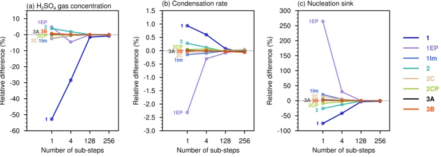
Fig. 2. Convergence plots for the globally integrated annual mean H2SO4gas (a) concentration, (b) condensation rate, and (c) loss rate due to aerosol nucleation, showing the relative differences with regard to reference solution, given by different time stepping schemes and numbers of sub-steps used for integrating the sulfuric acid equation (Eq. 1). The numerical schemes noted by labels in the figure are described in Table 1 and Sect. 2.2. The reference solution is established in Sect. 3.

gas loading down to a satisfactory level. In the new model version, such cancellation between physical and numerical errors no longer exists. In order to constrain the H2SO4gas loading in HAM2, it will probably be useful to re-evaluate the H2SO4 gas production and related parameterizations in ECHAM-HAM.

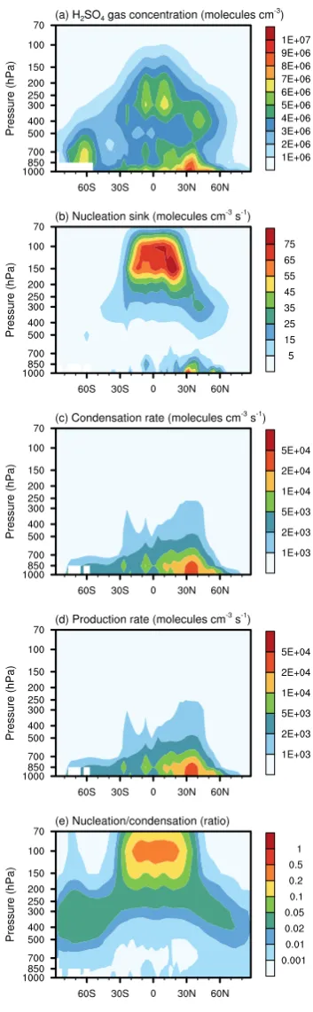
In the following sections, further analyses of the simula-tions shown in Table 1 and Fig. 2 are presented. Before go-ing into the details, we show in Fig. 3 the zonal and annual mean vertical cross sections of the H2SO4gas concentration as well as its source and sinks. The main locations of sul-fate particle formation are the tropical tropopause (Fig. 3b),

where high relative humidity and low temperature provide favorable conditions for the neutral nucleation of H2SO4and H2O, and the near-surface layers (Fig. 3b) where the con-centrations of H2SO4gas are high. Chemical production and condensation of the H2SO4gas peak in the near-surface lev-els where both the precursors and aerosol particles are abun-dant.

(7)

a typical case in numerical modeling where computational error easily contaminates the results. Further discussions on this issue are included in Sect. 4. In the tropical tropopause, nucleation plays a non-negligible role in the H2SO4gas bud-get where its magnitude can exceed 20 % of that of conden-sation in terms of annual and zonal mean (Fig. 3e). In this region, the partitioning of available sulfuric acid gas between condensation and nucleation, or in other words, the competi-tion between the two processes, becomes important for an ac-curate representation of nucleation. This is further discussed in Sect. 5.

4 Sulfuric acid gas concentration

4.1 Operator splitting

Based on the previous section, we can now explain the in-crease of H2SO4 gas concentration from Fig. 1a, b. The key reason is the replacement of a sequential splitting be-tween production and condensation by the analytical solution (Eq. 5) of the production-condensation equation.

In the real atmosphere, production and condensation oc-cur simultaneously. Condensation prevents H2SO4gas from linearly increasing, and forces it to asymptotically approach the equilibrium concentrationP /Cwith an e-folding time of C−1(cf. Eq. 5). A sequential splitting scheme first updates H2SO4gas by considering only the production, resulting in a positive error in the intermediate concentration that is used for computing the condensation rate. The scheme thus fea-tures systematic overestimate of condensation and negative bias in H2SO4gas burden, as can been seen in Fig. 2a, b (dark blue lines). The discretization errors are particularly large when the integration time step is long in comparison to the condensation time scale.

To verify this reasoning, we carried out two simulations, 1EP and 1Im, and compare them with simulation 1. The explicit parallel splitting of production and condensation is based on the thinking that since the two terms are largely compensating each other, the gas concentration will not change dramatically in one time step, thus the step-average concentration can be approximated by the initial value (Euler forward scheme, first-order accuracy). Parallel splitting re-duces the absolute error in H2SO4gas burden by a factor of 10 (Fig. 2a, purple vs. dark blue line). However, the conden-sation rate features a considerable negative bias (Fig. 2b, pur-ple line) because the condensation of newly produced H2SO4 gas is not considered. The implicit scheme, in contrast, con-siders production and condensation together, and approxi-mates the step-average concentration by the arithmetic av-erage of the initial and ending values. This method turns out much more accurate than schemes 1 and 1EP. The globally and annually averaged H2SO4gas concentration and conden-sation rate are very close to those obtained with the analytical solution (Fig. 2a, b, scheme 1Im vs. 2C).

(8)

Fig. 4. Reference solution of the January-mean H₂SO₄gas conden-sation coefficient (unit: s−1) in the lowest model layer. The numbers given in parentheses next to the color bar are the step sizes corre-sponding to the stability threshold1t=2/Cof the Euler forward time integration scheme (cf., e.g., Chapter 2 in Butcher, 2008).

These results suggest that for strongly compensating pro-cesses, both sequential and parallel splitting can lead to large numerical errors when used in combination with long time steps. Although our simulations 1 and 1EP both use Euler forward time stepping, the explicit nature of the schemes is not the main cause of errors in this case. In the aerosol module MAM3 of the CAM5 model (Liu et al., 2012), the production-condensation equation is solved with a sequen-tial splitting method like in HAM1, but using the analytical solution of the condensation equation dS/dt= −C·S, i.e., Eq. (3) is replaced by

S∗∗=S∗e−C1t. (19)

Despite the fact that Eqs. (2) and (19) are exact solutions of the production and condensation equations, respectively, results from the MAM3 module also have severe negative biases in H2SO4 gas concentration in the near-surface lev-els (Liu and Easter, personal communication, 2012). The real culprit of the systematic errors in our simulations 1, 1EP and in MAM3 is the use of operator splitting with a large time step. The HAM2 method and the implicit scheme 1Im solve production and condensation together, thus produce more ac-curate results.

4.2 Comments on sub-stepping and clipping

Many of the parameterization schemes in contemporary cli-mate models are nonlinear, which can make it impractical or inconvenient to use analytical solutions and/or implicit meth-ods. In such cases, sub-stepping is often used to handle fast processes. Here we want to point out several caveats related to the use of sub-stepping.

In Fig. 2a, the H2SO4 gas burden errors obtained with scheme 1EP are of opposite signs when 1 and 4 sub-steps are used. This reflects the inherent nature of the explicit scheme. According to the stability analysis in, e.g., Chapter 2 of Butcher (2008), the Euler forward scheme leads to oscilla-tory behavior in the solution of the production-condensation equation when the step size exceeds the e-folding time 1/C,

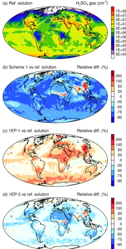
Fig. 5. (a) Reference solution of the January-mean near-surface H2SO4 gas concentration (unit: molecules per cm3). (b–d) Rela-tive differences with regard to the reference solution in simulations using scheme 1 (cf. Sect. 2.2), and using scheme 1EP without and with 2 sub-steps. All panels are plotted for the lowest model level. Similar figures of the other months convey the same message, al-though the spatial distributions are different because of the seasonal cycle.

(9)

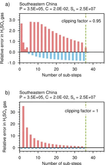
Fig. 6. Relative errors of H2SO4gas concentration in box model calculations that solve the production-condensation equation using the Euler forward scheme for an 1 h integration time. Typical val-ues of the production rateP, condensation coefficientC, and initial valueS0in Southeast China are used, which represents region asso-ciated with persistent positive errors in Fig. 5b–e. The dashed green line indicate the stability threshold1t=2/C(cf., e.g., Chapter 2 in Butcher, 2008). In panel (a) the estimated condensation rate at each step of time integration is limited to 95 % of the total available H2SO4gas, while in panel (b) this clipping factor is set to 1. Note that the two panels use different scales for the y-axis. Further details can be found in Sect. 4.2.

methods, e.g., Runge–Kutta and explicit predictor-corrector methods. Sensitivity experiments have been performed but are not shown here.

To reduce the errors, sub-stepping is needed to ensure suf-ficiently small step size. In current climate models, this is commonly employed with a fixed number of steps deter-mined by investigations of simplified test cases or evaluation of zonal mean statistics (e.g., Posselt and Lohmann, 2008; Morrison and Gettelman, 2008; Gettelman et al., 2008). In our simulations with the 1EP scheme, 8 sub-steps (7.5 min sub-step size) turns out sufficient to provide a less than 2 % error in the annual mean H2SO4gas burden, and less than 15 % errors in the annually averaged zonal mean concen-tration. However, the instantaneous values of condensation coefficients can be so high as to require more than 200 sub-steps. This is problematic for studies that use a fixed small number of sub-steps in applications that investigate

re-gional features and impacts. Given that very small step sizes (e.g., on the order of seconds) are expensive to use globally and also unnecessary for grid points with relatively weak condensation, the use of dynamically controlled time steps is worth considering. Zaveri et al. (2008) developed an adap-tive time stepping scheme using a priori estimates of step size, while Herzog et al. (2004) used time steps dynamically adjusted according to an a posteriori error estimate.

For the H2SO4gas equation in ECHAM-HAM, we tested a version of the 1EP scheme in which the sub-step size is calculated from the condensation coefficient. The number of sub-steps is chosen such that the stability factorC1t does not exceed unity. In order to stay with the original coding structure in ECHAM-HAM, the same number of sub-steps is applied to all grid boxes in the same CPU, determined by the largest condensation coefficient among these grid boxes. Results show that for a one-year simulation, the globally av-eraged number of sub-steps is about 20 when using 32 CPUs. The simulated annual mean H2SO4gas burden and conden-sation rate are less than 1 % different from the reference so-lution.

As a side remark, we note that the use of adaptive sub-stepping can cause load balancing issues in parallel comput-ing, when the same number of grid boxes are assigned to each CPU. This was not a problem in our simulations because the H2SO4 gas equation only took a very small fraction of the total computing time. The boundary layer nucleation scheme has a rather simple formulation, and the Kazil and Lovejoy (2007) parameterization is implemented as a look-up table (Kazil et al., 2010). For more complex and computation-ally expensive parameterization-like cloud macro- and mi-crophysics, the load imbalance can be significant or even be-come a bottle neck in parallelization. In such a case, the use of advanced domain decomposition algorithms, such as the METIS graph partitioning tool (Karypis and Kumar, 1995, 1998), will probably be helpful.

(10)

to a severely underestimated condensation rate in the next (sub-)step. The comparison of Fig. 6a with b suggests that the 95 % clipping factor does help to reduce errors in the heavily polluted regions when a small number of sub-steps are used. On the other hand, additional box model calculations (not shown) and the error patterns displayed in Fig. 5 indicate that the sign and magnitude of the errors depend on the charac-teristic condensation coefficient, thus have a strong regional variation. This again would undermine the accuracy of stud-ies that used such a clipping when studying regional features and impacts. To reduce the impact of clipping, smaller time steps and/or more accurate time integration schemes should be applied.

5 Aerosol nucleation and cloud condensation nuclei

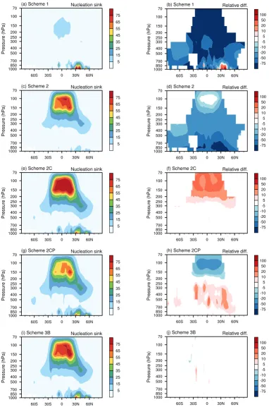
Numerical error in the simulated H2SO4gas nucleation sink comes from two sources: (i) the H2SO4 gas concentration provided as input to the nucleation parameterization scheme, e.g., S∗∗ in Eq. (4); and (ii) the time integration method used for the nucleation process, e.g., the correction factor 1/(1+C1t )in Eq. (6). The first source explains the 75 % negative bias in global mean nucleation sink given by the HAM1 numerics (scheme 1 in Fig. 2c, dark blue line), as well as the positive biases in the near-surface levels that can be seen from the zonally and annually averaged vertical cross section in Fig. 7b. The impact of source (ii) can be investi-gated by comparing schemes 2, 2C and 2CP in Table 1, in which the same numerical treatment is applied to production and condensation, while the coupling with nucleation is var-ied. The simulated zonal and annual mean nucleation sink is shown in Fig. 7c–h.

Scheme 2C applies a sequential splitting between production-condensation and nucleation (like in HAM2), but no special correction for nucleation. In regions where nucle-ation is non-negligible in magnitude (cf. Fig. 3e), the inter-mediate H2SO4gas concentrationS∗calculated with Eq. (5) (which ignores the nucleation sink) tends to have consider-able positive biases, resulting in overpredicted nucleation. This is why the scheme produces positive bias in the nucle-ation sink near the tropopause (Fig. 7e, f).

The nucleation adjustment factor 1/ (1+C1t ) that Kokkola et al. (2009) introduced to HAM2 (scheme 2, Eq. 6) helps to reduce the absolute bias in the upper troposphere, but tends to cause over-correction (negative biases in Fig. 7c, d). From the perspective of competition between condensation and nucleation, the HAM2 scheme favors condensation be-cause while the nucleation sink is scaled down, the condensa-tion process does not have any competitor in the first step of the calculation. The nucleation adjustment factor causes con-siderable negative biases in aerosol nucleation in the lower troposphere (Fig. 7d) due to the large condensation coeffi-cients and long time step. Close to the surface, the relative differences with regard to reference solution exceed−50 %

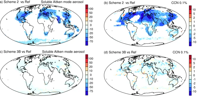
in middle and low latitudes, and even−75 % in polluted re-gions. Consequently, not only the concentration of the nu-cleation mode aerosols are severely underestimated, but also the Aitken mode number concentration is associated with biases of about 20 %–70 % in North America, Europe and North Africa, and in East Asia. The latter can be seen in Fig. 8a, where the relative errors in the Aitken mode num-ber concentration of the lowest model level are shown for scheme 2. The negative biases in the concentration of cloud condensation nuclei (CCN, diagnosed at 0.1 % supersatura-tion) generally exceed 5 % in these regions (Fig. 8b). Based on these results, we suggest removing the nucleation adjust-ment factor in future versions of the ECHAM-HAM model.

Without the adjustment factor (i.e., scheme 2C, Fig. 7f), the model provides good results in the near-surface levels but about 20 % relative errors in the nucleation sink near the tropical tropopause. If parallel splitting is applied between nucleation and production-condensation (scheme 2CP), er-rors of similar magnitude are produced although the signs are different (Fig. 7h). The time integration schemes 3A and 3B, which handle the three processes simultaneously, signif-icantly improves the nucleation sink throughout the model domain. Despite the fact that scheme 3B has the same order of accuracy (first-order) as those using sequential splitting, it produces smaller errors (Figs. 7j and 8c, d). Results from the second-order scheme 3A are similar to 3B, hence not shown. Because the purpose of solving the H2SO4gas equa-tion in ECHAM-HAM is to represent its impact on aerosol formation and growth, based on Figs. 7 and 8 we consider schemes 3A and 3B as better choices for this model.

As pointed out earlier in Sect. 3, the H2SO4gas budget in the middle and upper troposphere can be understood as the balance between nucleation (sink) and the residual of pro-duction minus condensation (source). The small errors asso-ciated with scheme 3B indicate again that strongly compen-sating processes need to be treated together by the numerical solver.

6 Conclusions

(11)

(12)

Fig. 8. Relative differences with regard to to the reference solution (unit: %) of the annual mean number concentrations of the soluble Aitken mode aerosol (left column) and the cloud condensation nuclei at 0.1 % supersaturation (CCN 0.1 %, right column) in the lowest model layer. The values are plotted only in regions with Aitken mode concentration>500 cm−3STP and CCN>50 cm−3, respectively. STP stands for standard temperature and pressure (1013.25 hPa, 273.15 K). The upper row shows results obtained with time integration scheme 2. The lower row corresponds to scheme 3B.

may have degraded from HAM1 to HAM2, our results in-dicate that the time stepping method should not be reverted. Instead, other components of the model, possibly the produc-tion of the H2SO4gas, need to be re-evaluated.

The time stepping scheme currently used in HAM2 in-cludes a numerical adjustment for the H2SO4 gas loss rate due to nucleation, which causes significant negative biases in the nucleation sink, aerosol number concentration, and CCN concentration in regions of strong condensation. We suggest this adjustment be removed in the future. Furthermore, two time stepping schemes based on the linearization of nucle-ation are tested in the paper. The schemes solve H2SO4gas production, condensation and nucleation simultaneously, and provide more accurate results than the current model version. In modern climate models that include process-based physics parameterizations, the wide spectrum of timescales poses new challenges to the numerical methods. Our study demonstrates that in situations involving strongly compen-sating and/or competing processes, operator splitting in com-bination with long time step can cause severe numerical er-rors. The sub-stepping technique used with a fixed small number of sub-steps may give good results in terms of global or zonal mean, but can still cause large regional biases due to the extremely short characteristic timescales in certain re-gions.

The key conclusion from this work is that, in order to reduce the biases associated with process interactions, it is important to apply numerical methods that solve multiple processes simultaneously. Such methods, employed together with implicit time stepping, can provide high-accuracy

re-sults without the need for very short time steps. As for sub-stepping, the use of dynamically adjusted step size can be beneficial, and provide a good trade-off between numerical accuracy and computational efficiency. The potential issue of load balancing in parallel computing may be addressed by advanced domain decomposition algorithms.

Acknowledgements. The authors thank Harri Kokkola (FMI), Xiaohong Liu (PNNL), Dick Easter (PNNL), Peter Caldwell (LLNL), Declan O’Donnell (FMI), Philip Stier (Oxford University) and Stefan Kinne (MPI-M) for valuable discussions. We also thank Luca Bonaventura and an anonymous reviewer, whose comments helped to improve the paper. H. Wan is grateful for the support of the Linus Pauling Distinguished Postdoctoral Fellowship of the Pacific Northwest National Laboratory (PNNL), a multiprogram laboratory operated for the US Department of Energy (DOE) by Battelle Memorial Institute under contract DE-AC05-76RL01830. The study described in this paper was conducted under the PNNL Laboratory Directed Research and Development Program. P. J. Rasch was supported by the DOE Office of Science as part of the Earth System Modeling Program (the Aerosol Clouds and Precipitation Science Focus Area), and the Scientific Discovery Through Advanced Computing (SciDAC) project on Multiscale Methods for Accurate, Efficient, and Scale-Aware Models of the Earth System. The ECHAM-HAM simulations presented in this paper were performed at the German Climate Computing Center (Deutsches Klimarechenzentrum, DKRZ).

(13)

References

Beljaars, A.: Numerical schemes for parameterizations, in: Numer-ical Methods in Atmospheric Models, ECMWF Seminar pro-ceedings, European Centre for Medium-range Weather Forecast, Reading, UK, 1–42, 1991.

Beljaars, A., Bechtold, P., Koehler, M., Morcrette, J.-J., Tomp-kins, A., Viterbo, P., and Wedi, N.: The numerics of physical parameterization, in: ECMWF Seminar Proceedings, European Centre for Medium-range Weather Forecast, Reading, UK, 113– 134, 2004.

Benard, P., Marki, A., Neytchev, P., and Prtenjak, M.: Stabilization of nonlinear vertical diffusion schemes in the context of NWP models, Mon. Wea. Rev., 128, 1937–1948, doi:10.1175/1520-0493(2000)128<1937:SONVDS>2.0.CO;2, 2000.

Brinkop, S. and Roeckner, E.: Sensitivity of a general circula-tionmodel to parameterizations of cloud-turbulence interactions inthe atmospheric boundary layer, Tellus A, 47, 197–220, 1995. Butcher, J. C.: Numerical methods for ordinary differential

equa-tions, John Wiley & Sons Ltd., 2nd edn., 2008.

Cheng, T., Peng, Y., Feichter, J., and Tegen, I.: An improve-ment on the dust emission scheme in the global aerosol-climate model ECHAM5-HAM, Atmos. Chem. Phys., 8, 1105–1117, doi:10.5194/acp-8-1105-2008, 2008.

Dentener, F., Kinne, S., Bond, T., Boucher, O., Cofala, J., Gen-eroso, S., Ginoux, P., Gong, S., Hoelzemann, J. J., Ito, A., Marelli, L., Penner, J. E., Putaud, J.-P., Textor, C., Schulz, M., van der Werf, G. R., and Wilson, J.: Emissions of primary aerosol and precursor gases in the years 2000 and 1750 pre-scribed data-sets for AeroCom, Atmos. Chem. Phys., 6, 4321– 4344, doi:10.5194/acp-6-4321-2006, 2006.

Fouquart, Y. and Bonnel, B.: Computations of solar heating of the earth’s atmosphere: a new parameterization., Phys. Atmos., 53, 35–62, 1980.

Gettelman, A., Morrison, H., and Ghan, S. J.: A new two-moment bulk stratiform cloud microphysics scheme in the Community Atmospheric Model (CAM3), Part II: Single-column and global results, J. Climate, 21, 3660–3679, 2008.

Girard, C. and Delage, Y.: Stable schemes for nonlin-ear vertical diffusion in atmospheric circulation models, Mon. Weather Rev., 118, 737–745, doi:10.1175/1520-0493(1990)118<0737:SSFNVD>2.0.CO;2, 1990.

Hairer, E. and Wanner, G.: Solving ordinary differential equations II: Stiff and differential-algebraic problems, Springer, 2nd edn., 2004.

Herzog, M., Weisenstein, D. K., and Penner, J. E.: A dy-namic aerosol module for global chemical transport mod-els: model description, J. Geophys. Res., 109, D18202, doi:10.1029/2003JD004405, 2004.

Hochbruck, M., Ostermann, A., and Schweitzer, J.: Exponential Rosenbrock-Type Methods, SIAM J. Numer. Anal., 47, 786–803, doi:10.1137/080717717, 2009.

Jacobson, M. Z.: Analysis of aerosol interactions with nu-merical techniques for solving coagulation, nucleation, condensation, dissolution, and reversible chemistry among multiple size distributions., J. Geophys. Res., 107, 4366, doi:10.1029/2001JD002044, 2002.

Jacobson, M. Z.: Fundamentals of atmospheric modeling, Cam-bridge University Press, 2nd edn., 2005.

Karypis, G. and Kumar, V.: Multilevel graph partitioning schemes, in: International Conference on Parallel Processing, 1995. Karypis, G. and Kumar, V.: A fast and high quality multilevel

scheme for partitioning irregular graphs, SIAM J. Sci. Comput., 20, 359–392, doi:10.1137/S1064827595287997, 1998.

Kazil, J. and Lovejoy, E. R.: A semi-analytical method for calculat-ing rates of new sulfate aerosol formation from the gas phase, At-mos. Chem. Phys., 7, 3447–3459, doi:10.5194/acp-7-3447-2007, 2007.

Kazil, J., Stier, P., Zhang, K., Quaas, J., Kinne, S., O’Donnell, D., Rast, S., Esch, M., Ferrachat, S., Lohmann, U., and Feichter, J.: Aerosol nucleation and its role for clouds and Earth’s ra-diative forcing in the aerosol-climate model ECHAM5-HAM, Atmos. Chem. Phys., 10, 10733–10752, doi:10.5194/acp-10-10733-2010, 2010.

Kerkweg, A., Buchholz, J., Ganzeveld, L., Pozzer, A., Tost, H., and J¨ockel, P.: Technical Note: An implementation of the dry removal processes DRY DEPosition and SEDImentation in the Modu-lar Earth Submodel System (MESSy), Atmos. Chem. Phys., 6, 4617–4632, doi:10.5194/acp-6-4617-2006, 2006.

Kokkola, H., Hommel, R., Kazil, J., Niemeier, U., Partanen, A.-I., Feichter, J., and Timmreck, C.: Aerosol microphysics modules in the framework of the ECHAM5 climate model – intercomparison under stratospheric conditions, Geosci. Model Dev., 2, 97–112, doi:10.5194/gmd-2-97-2009, 2009.

Kuang, C., McMurry, P. H., McCormick, A. V., and Eisele, F. L.: Dependence of nucleation rates on sulfuric acid vapor concen-tration in diverse atmospheric locations, J. Geophys. Res., 113, D10209, doi:10.1029/2007JD009253, 2008.

Kulmala, M., Lehtinen, K. E. J., and Laaksonen, A.: Cluster activa-tion theory as an explanaactiva-tion of the linear dependence between formation rate of 3nm particles and sulphuric acid concentration, Atmos. Chem. Phys., 6, 787–793, doi:10.5194/acp-6-787-2006, 2006.

Laakso, L., Petäjä, T., Lehtinen, K. E. J., Kulmala, M., Paatero, J., Hõrrak, U., T ammet, H., and Joutsensaari, J.: Ion production rate in a boreal forest based on ion, particle and radiation measure-ments, Atmos. Chem. Phys., 4, 1933–1943, doi:10.5194/acp-4-1933-2004, 2004.

Lin, S.-J. and Rood, R. B.: Multidimensional flux-form semi-Lagrangian transport schemes, Mon. Weather Rev., 124, 2046– 2070, 1996.

Liu, X., Easter, R. C., Ghan, S. J., Zaveri, R., Rasch, P., Shi, X., Lamarque, J.-F., Gettelman, A., Morrison, H., Vitt, F., Con-ley, A., Park, S., Neale, R., Hannay, C., Ekman, A. M. L., Hess, P., Mahowald, N., Collins, W., Iacono, M. J., Brether-ton, C. S., Flanner, M. G., and Mitchell, D.: Toward a min-imal representation of aerosols in climate models: description and evaluation in the Community Atmosphere Model CAM5, Geosci. Model Dev., 5, 709–739, doi:10.5194/gmd-5-709-2012, 2012.

Lohmann, U. and Hoose, C.: Sensitivity studies of different aerosol indirect effects in mixed-phase clouds, Atmos. Chem. Phys., 9, 8917–8934, doi:10.5194/acp-9-8917-2009, 2009.

(14)

Mlawer, E. J., Taubman, S. J., Brown, P. D., Iacono, M. J., and Clough, S. A.: Radiative transfer for inhomogeneous atmo-spheres: RRTM, a validated correlated-k model for the long-wave., J. Geophys. Res., 102, 16663–16682, 1997.

Monahan, E., Spiel, D., and Davidson, K.: A model of ma-rine aerosol generation via whitecaps and wave disruption, in: Oceanic Whitecaps and their Role in Air-Sea Exchange, edited by: Reidel, D., Norwell, Massachusetts, 167–174, 1986. Morrison, H. and Gettelman, A.: A new two-moment bulk

strat-iform cloud microphysics scheme in the Community Atmo-spheric Model (CAM3), Part I: Description and numerical tests, J. Climate, 21, 3642–3659, 2008.

Nordeng, T. E.: Extended versions of the convective parametriza-tion scheme at ECMWF and their impact on the mean and tran-sient activity of the model in the tropics, ECMWF Research Department, Technical Momorandum 206, European Centre for Medium-range Weather Forecast, Reading, UK, Reading, UK, 1994.

O’Donnell, D., Tsigaridis, K., and Feichter, J.: Estimating the direct and indirect effects of secondary organic aerosols us-ing ECHAM5-HAM, Atmos. Chem. Phys., 11, 8635–8659, doi:10.5194/acp-11-8635-2011, 2011.

Petters, M. D. and Kreidenweis, S. M.: A single parameter repre-sentation of hygroscopic growth and cloud condensation nucleus activity, Atmos. Chem. Phys., 7, 1961–1971, doi:10.5194/acp-7-1961-2007, 2007.

Posselt, R. and Lohmann, U.: Introduction of prognostic rain in ECHAM5: design and single column model simulations, At-mos. Chem. Phys., 8, 2949–2963, doi:10.5194/acp-8-2949-2008, 2008.

Riipinen, I., Sihto, S.-L., Kulmala, M., Arnold, F., Dal Maso, M., Birmili, W., Saarnio, K., Teinilä, K., Kerminen, V.-M., Laak-sonen, A., and Lehtinen, K. E. J.: Connections between atmo-spheric sulphuric acid and new particle formation during QUEST III–IV campaigns in Heidelberg and Hyytiälä, Atmos. Chem. Phys., 7, 1899–1914, doi:10.5194/acp-7-1899-2007, 2007. Roeckner, E., Bäuml, G., Bonaventura, L., Brokopf, R., Esch, M.,

Giorgetta, M., Hagemann, S., Kirchner, I., Kornblueh, L., Manzini, E., Rhodin, A., Schlese, U., Schulzweida, U., and Tompkins, A.: The atmospheric general circulation model ECHAM5. PART I: model description, Technical Report 349, Max Planck Institute for Meteorology, 2003.

Roeckner, E., Brokopf, R., Esch, M., Giorgetta, M., Hagemann, S., Kornblueh, L., Manzini, E., Schlese, U., and Schulzweida, U.: Sensitivity of simulated climate to horizontal and vertical reso-lution in the ECHAM5 atmosphere model, J. Climate, 19, 3771– 3791, 2006.

Rosenbrock, H. H.: Some general implicit processes for the numer-ical solution of differential equations, The Computer Journal, 5, 329–330, doi:10.1093/comjnl/5.4.329, 1963.

Schlegel, M., Knoth, O., Arnold, M., and Wolke, R.: Implementa-tion of multirate time integraImplementa-tion methods for air polluImplementa-tion mod-elling, Geosci. Model Dev., 5, 1395–1405, doi:10.5194/gmd-5-1395-2012, 2012.

Schweitzer, J.: The exponential Rosenbrock-Euler method for non-smooth initial data, Numer. Math., in press, 2013.

Simmons, A. J. and Burridge, D. M.: An energy and angular-momentum conserving vertical finite difference scheme and hy-brid vertical coordinates, Mon. Weather Rev., 109, 758–766,

1981.

Smith, M. and Harrison, N.: The sea spray generation function., J. Aerosol Sci., 29, 189–190, doi:10.1016/S0021-8502(98)00280-8, 1998.

Stier, P., Feichter, J., Kinne, S., Kloster, S., Vignati, E., Wilson, J., Ganzeveld, L., Tegen, I., Werner, M., Balkanski, Y., Schulz, M., Boucher, O., Minikin, A., and Petzold, A.: The aerosol-climate model ECHAM5-HAM, Atmos. Chem. Phys., 5, 1125–1156, doi:10.5194/acp-5-1125-2005, 2005.

Tegen, I., Harrison, S. P., Kohfeld, K., Prentice, I. C., Coe, M., and Heimann, M.: Impact of vegetation and preferential source areas on global dust aerosol: results from a model study., J. Geophys. Res., 107, 4576–4597, doi:10.1029/2001JD000963, 2002. Teixeira, J.: Boundary layer clouds in large scale atmospheric

mod-els: cloud schemes and numerical aspects, Phd thesis, European Centre for Medium-range Weather Forecast, Reading, UK, 2000. Tiedtke, M.: A comprehensive mass flux scheme for cumulus pa-rameterization in large scale models, Mon. Weather Rev., 117, 1779–1800, 1989.

Tudor, M.: A test of numerical instability and stiffness in the parametrizations of the ARP ´EGE and ALADIN models, Geosci. Model Dev. Discuss., 5, 4233–4268, doi:10.5194/gmdd-5-4233-2012, 2012.

Uppala, S. M., Kallberg, P. W., Simmons, A. J., Andrae, U., Bech-told, V. D. C., Fiorino, M., Gibson, J. K., Haseler, J., Hernan-dez, A., Kelly, G. A., Li, X., Onogi, K., Saarinen, S., Sokka, N., Allan, R. P., Andersson, E., Arpe, K., Balmaseda, M. A., Bel-jaars, A. C. M., Berg, L. V. D., Bidlot, J., Bormann, N., Caires, S., Chevallier, F., Dethof, A., Dragosavac, M., Fisher, M., Fuentes, M., Hagemann, S., Holm, E., Hoskins, B. J., Isaksen, L., Janssen, P. A. E. M., Jenne, R., Mcnally, A. P., Mahfouf, J.-F., Morcrette, J.-J., Rayner, N. A., Saunders, R. W., Simon, P., Sterl, A., Trenberth, K. E., Untch, A., Vasiljevic, D., Viterbo, P., and Woollen, J.: The ERA-40 re-analysis, Q. J. Roy. Meteor. Soc., 131, 2961–3012, doi:10.1256/qj.04.176, 2005.

Vignati, E., Wilson, J., and Stier, P.: M7: An efficient size-resolved aerosol microphysics module for large-scale aerosol transport models., J. Geophys. Res., 109, D22202, doi:10.1029/2003JD004485, 2004.

Wood, N., Diamantakis, M., and Staniforth, A.: A monotonically-damping second-order-accurate unconditionally-stable numeri-cal scheme for diffusion, Q. J. Roy. Meteor. Soc., 133, 1559– 1573, doi:10.1002/qj.116, 2007.

Zaveri, R. A., Easter, R. C., Fast, J. D., and Peters, L. K.: Model for Simulating Aerosol Interactions and Chem-istry (MOSAIC), J. Geophys. Res.-Atmos., 113, D13204, doi:10.1029/2007JD008782, 2008.

Zhang, K., Wan, H., Wang, B., Zhang, M., Feichter, J., and Liu, X.: Tropospheric aerosol size distributions simulated by three on-line global aerosol models using the M7 microphysics module, Atmos. Chem. Phys., 10, 6409–6434, doi:10.5194/acp-10-6409-2010, 2010.