University of Trento
Alessia Ussia (Ph.D. Student)
INPUT IDENTIFICATION, FOOTBRIDGE
CONTROL AND NON-LINEAR
IDENTIFICATION OF A MR DAMPER
Prof. Oreste S. Bursi (Tutor)
University of Trento
Doctorate in Engineering of Civil and Mechanical
Structural Systems - Cycle XXVI
Board of examiners:
Prof. Dionisio P. Bernal
Prof. Michel Destrade
Prof. Oreste S. Bursi
Prof. Andrea G. Calogero
ABSTRACT
ACKNOLEDGEMENTS
Vorrei ringraziare in primis i miei genitori per il sostegno sempre presente, poi il Prof. Bursi per la grande opportunita’, Alessio per l’estrema disponibilita’
dimostrata
e tutti quelli con con cui ho lavorato e collaborato in questi anni.
CONTENTS
1 INTRODUCTION 1
1.1 Motivation . . . 1
1.2 Organization of the thesis . . . 3
1.3 Objectives . . . 4
2 STATE SPACE REPRESENTATION, OBSERVERS AND CONTROLLERS 5 2.1 Introduction . . . 5
2.2 Continuous time state space representation . . . 5
2.2.1 Response to a general input . . . 7
2.3 Discrete time state-space representation . . . 8
2.3.1 Zero order hold . . . 10
2.3.2 First order hold . . . 11
2.4 Observability, reconstructability and detectability . . . 15
2.4.1 The initial condition issue . . . 18
2.4.2 Closed loop asymptotic estimator . . . 19
2.5 Dynamic response and Markov parameters . . . 20
2.6 LQR and LQG controller . . . 21
2.6.1 LQR in continuous time and finite/infinite horizon . . . 21
2.6.2 LQR in discrete time and finite/infinite horizon . . . 22
2.7 Modal domain . . . 23
2.8 Model reduction . . . 24
3 THE KALMAN FILTER THEORY FOR INPUT AND STATE ESTIMATION 27 3.1 Introduction . . . 27
3.2.1 The state estimator . . . 29
3.2.2 Innovation form of the Filter . . . 31
3.2.3 The steady state form of the Filter . . . 32
3.2.4 The Kalman-Bucy filter . . . 33
3.3 The Kalman Filter for input identification . . . 34
3.3.1 RLS approach . . . 35
3.3.2 Minimum-Variance Unbiased input and state estimation al-gorithms . . . 37
3.3.3 The steady state observer method . . . 40
3.4 Introduction to non-linear filters . . . 41
3.4.1 The process to be estimated . . . 43
3.4.2 The Extended Kalman Filter . . . 43
3.4.3 The Unscented Transformation . . . 44
3.4.4 The Unscented Kalman Filter . . . 47
4 THE NOMI FOOTBRIDGE 49 4.1 Introduction . . . 49
4.2 Control of structures . . . 50
4.2.1 Passive control . . . 51
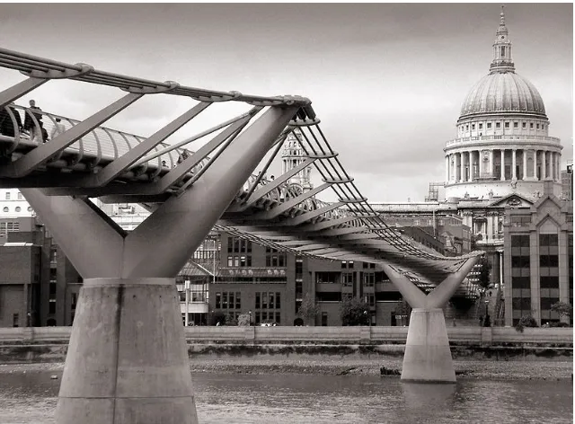
4.2.1.1 Millennium bridge . . . 52
4.2.1.2 San Michele all’Adige . . . 53
4.2.1.3 Ponte del Mare . . . 54
4.2.2 Active control . . . 55
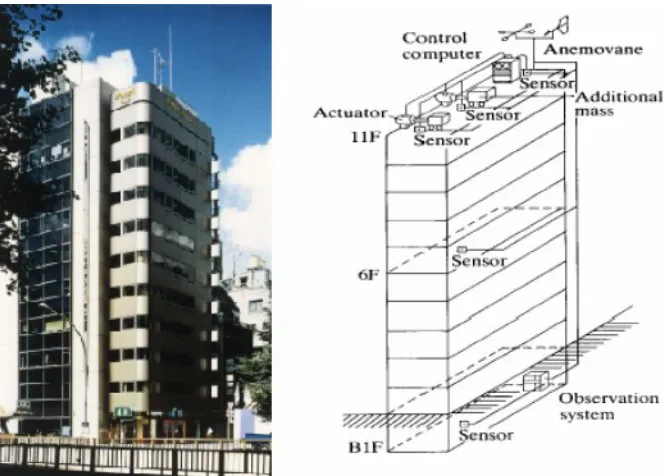
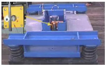
4.2.2.1 Kyobashi Building, 1989 . . . 57
4.2.2.2 Osaka ORC 200 Building, 1992 . . . 57
4.2.3 Semi-active control . . . 57
4.2.3.1 The Kajima Shinozuoka Building in Shinozuoka . . 58
4.2.3.2 The Bilbao footbridge . . . 60
4.2.3.3 Forcheim footbridge . . . 60
4.3 The Nomi Calliano footbridge design . . . 61
4.4 The FEM model . . . 63
4.5.1 Determination of the footbridge class according with Setra’
guide . . . 65
4.5.2 Determination of the resonant risk . . . 65
4.5.3 Choose of the comfort levels . . . 66
4.5.4 Load cases . . . 67
4.5.5 The soil stiffness . . . 68
4.5.6 Design loads . . . 72
4.6 Tuned Mass Damper . . . 74
4.6.1 The influence of the soil stiffness on the TMD design . . . 80
4.7 Experimental modal analysis and model updating . . . 84
4.7.1 Set-up . . . 84
4.7.2 Results . . . 86
4.7.3 Refinement and updating . . . 88
4.8 The damping system . . . 89
4.9 The monitoring system . . . 91
4.10 Conclusions . . . 93
5 INPUT IDENTIFICATION 97 5.1 Introduction . . . 97
5.2 Issues related to input identification . . . 98
5.2.1 The deconvolution approach . . . 101
5.2.2 Input-output relations in time-domain . . . 102
5.3 Number and location of inputs . . . 103
5.3.1 On the number . . . 104
5.3.2 On the location . . . 107
5.4 Identificability . . . 109
5.5 The segmented deconvolution algorithm . . . 116
5.6 Stability . . . 117
5.7 The Fisher information . . . 122
5.8 Conditioning in the frequency domain . . . 124
5.9 Conditioning in the time domain . . . 126
5.10 Singular Values Truncation . . . 128
5.11.1 Tests on number and position . . . 131
5.11.2 Tests on the time histories . . . 131
5.12 Conclusions . . . 132
5.13 Appendix A - Dead Time in Finite Dimensional Systems Impulse Response Functions . . . 134
5.14 Appendix B - Illustration of Vectors in 5.9 . . . 136
6 MODELING AND SEMI-ACTIVE CONTROL OF A MAGNETO-RHEOLOGICAL TUNED MASS DAMPER 139 6.1 Introduction . . . 139
6.2 Non-linear models for hysteretic systems . . . 140
6.2.1 The Bouc model . . . 141
6.2.2 The Wen model . . . 141
6.2.3 The Bouc-Wen model . . . 142
6.2.4 The Baber-Wen model . . . 143
6.2.5 The Baber-Noori model . . . 145
6.2.6 The Foliente model . . . 147
6.3 MR fluids and hysteresis mathematical models . . . 147
6.4 Non-linear identification of the MR damper . . . 151
6.4.1 MR damper and test description . . . 154
6.4.2 Parametric model of the damper and results . . . 159
6.5 The UKF for parameter identification . . . 165
6.5.1 Numerical benchmarks . . . 165
6.5.2 Experimental application to time invariant MR damper . . . . 169
6.6 Semi-active control . . . 170
6.6.1 Semi-active control strategies: state of the art . . . 172
6.6.2 Clipped optimal control in detail . . . 175
6.6.3 The model of the controlled structure . . . 179
6.6.4 Control concept applied to the simulated MR damper . . . 179
6.6.5 Experimental set-up on the footbridge . . . 182
6.6.6 Control validation . . . 185
6.7 Conclusions . . . 187
7 SUMMARY, CONCLUSIONS AND FUTURE PERSPECTIVES 193
7.1 Summary . . . 193
7.2 Conclusions . . . 194
7.3 Future perspectives . . . 197
LIST OF
FIGURES
2.1 system representation by means of block diagrams. . . 8
2.2 discrete and continuous signal. . . 11
2.3 Open loop state estimator. . . 18
2.4 closed loop asymptotic estimator. . . 19
3.1 state and input observer layout. . . 35
3.2 the Kalman observer. . . 35
3.3 the RLS observer. . . 37
3.4 The Unscented Transformation . . . 45
4.1 working layout of the passive device. . . 51
4.2 behavior of different types of dampers. . . 52
4.3 Millennium Bridge, London. . . 53
4.4 San Michele Footbridge. . . 54
4.5 Ponte del mare, Pescara. . . 55
4.6 a) and b) passive control system positioning; c) damper Type A and B; d) damper Type C. . . 56
4.7 working layout of active devices. . . 56
4.8 Kyobashi Building. . . 58
4.9 Osaka Building . . . 59
4.10 Kajima Shinozuka Building - semi-active hydraulic damper. . . 59
4.11 The Bilbao footbridge. . . 60
4.12 Forcheim footbridge, Munich . . . 61
4.13 Semi-active MR TMD. . . 61
4.14 the Nomi-Calliano footbridge. . . 62
4.16 frequency range for a) vertical/longitudinal and b) transverse
oscilla-tions. . . 66
4.17 a) vertical and b) horizontal limit for accelerations. . . 67
4.18 1st natural mode for a) Kminand b) Kmax . . . 70
4.19 2nd natural mode a) Kminand b) Kmax . . . 70
4.20 3rd natural mode a)Kminand b) Kmax . . . 71
4.21 4thnatural mode a) Kminand b) Kmax . . . 71
4.22 5thnatural mode a) Kminand b) Kmax . . . 71
4.23 single oscillator endowed with the mass damper . . . 76
4.24 behavior of the optimal design parameters for the TMD as function of the mass ratio. . . 78
4.25 dynamic amplification factors as function of a)the mass ratio and of b)the optimal damper stiffness. . . 79
4.26 dynamic amplification factors as function of the damping ratio of the damper for a)β̸= 1and b)β= 1 . . . 80
4.27 effects of the mistuning. . . 81
4.28 optimal stiffness of the TMD spring. . . 83
4.29 optimal damping of the TMD dashpot. . . 84
4.30 accelerometers set-up. . . 85
4.31 spectrogram referred to Ch.1 and generated by the test with the mass unfasten . . . 86
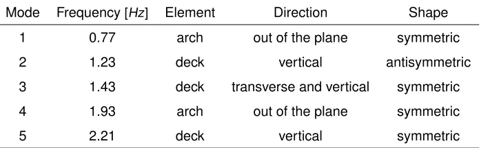
4.32 first five modes identified within the campain. . . 87
4.33 the disposition of the damping system on the footbridge. . . 90
4.34 acquisition 2013 11 11 04 14 47 AFW.txt, contribution of the 4thmode. 92 5.1 causes and effects on a structure. . . 97
5.2 input quantification in a) linear and b) logarithmic scale . . . 106
5.3 rank definition as a function of the window size. . . 107
5.6 example of non empty null space. . . 111
5.7 kernel of a 40-DoF chain system subjected to variation of the sensor location a) the model; b)SISO with the input in #40 and output on #1; and c) SISO with the input in #40 and output on #20. . . 113
5.8 kernel of a 40-DoF chain system subjected to variation of the sensor location: a) the model; b)SIMO with the input in #40 and outputs on #1 and #20; and c) SISO with the input in #40 and output on #20. . . 114
5.9 kernel of a 40-DoF chain system with inputs in position #5 and #40, a) the model; b) the kernel . . . 115
5.10 SDR algorithm . . . 117
5.11 relationship between radius of convergence and parameter p. . . . 121
5.12 radius of convergence and damping . . . 122
5.13 convergences problem: a) diverged solution, b) addition of a sensor, c) filtered identified input. . . 123
5.14 The dependence of Y on the parameterθ. . . . 124
5.15 the CRLB for a) not collocated; and b) collocated measurements. . . 126
5.16 example of bad conditioning in the frequency domain. . . 127
5.17 example of good conditioning in the frequency domain. . . 128
5.18 example of ill conditioning in the time domain. . . 129
5.19 effect of regularization on stability. . . 130
5.20 effect of regularization on conditioning in time domain. . . 130
5.21 the set-up of the experimental test on the beam. . . 131
5.22 number and position of independent inputs acting on the beam. . . . 131
5.23 conditioning in a) frequency; and b) time domain in the experimental test. . . 132
5.24 comparison between the actual and the predicted input. . . 133
6.1 increasing effect of the parameter n on: a) softening; and b) harden-ing hysteresis model (Heine, 2001). . . 144
6.2 pinching function for: a) the Baber-Noori and b) Foliente model (Foliente, 1995). . . 146
6.3 the Bingham model (Zapateiro De La Hoz, 2009) . . . 149
6.5 the Hyperbolic tangent model (Zapateiro De La Hoz, 2009) . . . 150
6.6 the Dahl friction model (Zapateiro De La Hoz, 2009) . . . 151
6.7 classification of non linear identification methods (Zanotti, 2012). . . 153
6.8 The TT1 sensor and plant set-up. . . 155
6.9 sketch of the Parker actuator. . . 156
6.10 the load cell TC4 25kN. . . 156
6.11 Control and acquisition instrumentation set-up in the TT1 Test rig. . 157
6.12 TT1 set-up for the damper identification. . . 159
6.13 model validation of the input dependent model. . . 162
6.14 model validation of the voltage dependent model. . . 165
6.15 Bouc-Wen model, comparison between: a) numerical and estimated hysteretic cycle; b) numerical and estimated restoring force. . . 167
6.16 parameters estimation of the Bouc-Wen model. . . 167
6.17 Baber-Noori model, comparison between: a) numerical and esti-mated hysteretic cycle; b) numerical and estiesti-mated restoring force. . . . 169
6.18 Baber Noori model; parameters estimation. . . 170
6.19 experimental test: comparison between measured and estimated hysteresis cycle. . . 172
6.20 comparison between measured and estimated: a)A ; b)β; and c)γ parameters. . . 173
6.21 a) sky-hook logic; and b) ground-hook logic. . . 174
6.22 the “Hook” logic. . . 175
6.23 the clipped logic. . . 177
6.24 LQG clipped control scheme. . . 178
6.25 2DoF models for preliminary tests: a) wo damper; b) optimal damper, c) Bouc-Wen-based damper; and d) forced system with clipped MR damper. . . 181
6.26 FRFs of the seven tested cases. . . 182
6.27 the instrumented damper within the TMD. . . 183
6.29 detailed scheme of instruments located on both the control room and the deck. . . 185 6.30 conditioning in the time domain of the 2DoF validation system. . . . 186 6.31 reconstructed and real modal accelerations for event #1. . . 187 6.32 plot of reduced accelerations for event #1 . . . 187 6.33 test with sinusoidal reference of 14 mm amplitude and subjected to
0V: a) Damper force time history; b) Force vs. Displacements cycle; and c) Force vs. Velocity cycle. . . 189 6.34 test with sinusoidal reference of 14 mm amplitude and subjected to
3V: a) Damper force time history; b) Force vs. Displacements cycle; and c) Force vs. Velocity cycle. . . 190 6.35 test with sinusoidal reference of 14 mm and 0.25 Hz: a) Damper
force time history; b) Force vs. Displacements cycle; and c) Force vs. Velocity cycle. . . 190 6.36 test with sinusoidal reference of 14 mm and 0.5 Hz: a) Damper force
time history; b) Force vs. Displacements cycle; and c) Force vs. Velocity cycle. . . 191 6.37 test with sinusoidal reference of 14 mm and 1 Hz: a) Damper force
time history; b) Force vs. Displacements cycle; and c) Force vs. Velocity cycle. . . 191 6.38 test with sinusoidal reference of 14 mm and 2 Hz: a) Damper force
LIST OF
TABLES
2.1 Closed form of the state matrices as function of the discrete
assump-tions on the input. . . 10
3.1 Discrete-Time filter equation. . . 33
3.2 RLS algorithm . . . 36
3.3 the steady state observer . . . 41
4.1 dampers characteristics, Ponte del Mare, Pescara - Italy. . . 55
4.2 frequency range for walking and running (Setra’, 2006). . . 64
4.3 density of the crowd. . . 65
4.4 maximum values for acceleration according to EN1990 (1990, 2006). 67 4.5 load cases. . . 68
4.6 natural frequencies as function of the soil stiffness. . . 69
4.7 Main characteristic of the first five modes for Kmin. . . 69
4.8 Main characteristic of the first five modes for Kmax. . . 70
4.9 maximum vertical acceleration for minimum soil stiffness. . . 74
4.10 maximum transverse acceleration for minimum soil stiffness. . . 74
4.11 maximum vertical acceleration for maximum soil stiffness. . . 75
4.12 maximum transverse acceleration for maximum soil stiffness. . . 75
4.13 frequency variation between identified and FEM modes. . . 89
4.14 estimated frequencies for TMD design. . . 90
4.15 TMD design. . . 95
5.1 k and k + p in the time line with p = 4. . . 119
6.2 typical MR fluid properties (Carlson et al., 1996; Carlson and Jolly,
2000). . . 148
6.3 specifications of the MR damper . . . 157
6.4 list of tests. . . 158
6.5 Values for parameters A ,βandγ. . . . 160
6.6 values of the parameterα0 . . . 162
6.7 test with 10 mm of the sine amplitude: optimized parameters. . . 163
6.8 test with 14 mm of the sine amplitude: optimized parameters. . . 164
6.9 numerical, initial and estimated values of the Bouc-Wen model pa-rameters. . . 168
6.10 numerical, initial and estimated values of the Baber-Noori model pa-rameters. . . 171
CHAPTER
1
INTRODUCTION
1.1 Motivation
used within the framework of a real application with the aim of validating the in-vestigated semi-active strategy. The reconstructed input is in fact applied on the simplified 2DoF model outlined by the Den Hartog theory and used in the design of the controller. The final result is that the validation of the control strategy took ad-vantage of both the recorded data from the monitoring system of the real structure and the input identification technique.
1.2 Organization of the thesis
This thesis presents the research proposed by the author on system identifica-tion and control of a MR damper together with a study on the input identificaidentifica-tion strategies. This research is sponsored by the Autonomous Province of Trento and includes the following chapters.
• Chapter 1presents the thesis objectives and motivation.
• Chapter 2is an introductory Chapter summarizing the linear time invariant systems theory. Both continuous and discrete time state space representa-tion of dynamical systems are introduced together with the concept of observ-ability and dynamic response in terms of Markov parameters. A brief portion of the control theory is reported with the description of the LQR algorithm. Eventually, both the modal domain representation and the order reduction of the system are presented.
• Chapter 3treats the Kalman Filter theory. The chapter is focused mainly on the linear filter and on its non linear version called Unscented Kalman Filter since they have been used within the input identification field. The in-depth analysis of references with respect to the Kalman filter application has highlighted some significant issues.
devices. At his purpose, dynamic identification and model updating are per-formed.
• Chapter 5 is dedicated to the input identification theory and to issues re-lated to the input reconstruction. The Segmented Deconvolution Algorithm is presented and validated by means of both numerical and experimental tests.
• Chapter 6is about testing, identification and semi-active control of the tuned mass damper with the aid of numerical and experimental tools such as the input reconstruction and real data.
• Chapter 7contains summary, conclusions and future perspectives.
1.3 Objectives
CHAPTER
2
STATE SPACE REPRESENTATION, OBSERVERS AND
CONTROLLERS
2.1 Introduction
In this chapter there are some basic concepts regarding the theory of the Linear Time Invariant systems (LTI). These systems are described in term of state space representation which is a mathematical model of a physic system composed by a set of inputs, outputs and state variables connected by first order differential equations. First, the continuous and the discrete space representation and their relation is reported and the hypothesis at the base of both the Zero Order Hold (ZOH) and the First Order Hold (FOH) discretization is described in detail. Then, the concepts of observability, reconstructability and detectability are introduced and more attention about the asymptotic state estimator in open and closed loop is payed. In addition, the dynamic properties of the LTI system are described in terms of Markov parameters. A brief description of Linear Quadratic Regulator (LQR) and Linear Quadratic Gaussian regulator (LQG) are reported and eventually, the system dynamic behavior is described in term of modal coordinates in state space and the concept of modal truncation is introduced.
2.2 Continuous time state space representation
The equation of motion for a finite dimensional linear dynamic system viscous damped in second order form is in Juang and Phan (2001) and can be described as,
where M, C and K∈Rnxnare the mass, damping and stiffness matrix, respectively. ¨
u(t), ˙u(t) and u(t)∈ Rn are the acceleration, velocity and displacement vector, re-spectively. S ∈ Rnxr gives the spatial distribution of the r excitations d(t) ∈ Rr. Assuming that M is invertible, one can write,
¨
u(t) =−M−1C ˙u(t)−M−1Ku(t) + M−1Sd(t) (2.2) Adding the equation ˙u(t) = ˙u(t), one has
d dt u(t) ˙ u(t) =
0 I
−M−1K −M−1C u(t) ˙ u(t) + 0
M−1S
d(t) (2.3)
where x(t) = x1(t)
x2(t) = u(t) ˙ u(t)
is the state vector and x(t)∈ R2n. Substituting the state vector into Eq. 2.1 one gets,
˙
x(t) = Acx(t) + Bcd(t) (2.4)
with the system matrix Ac ∈R2nx2n, where Ac =
0 I
−M−1K −M−1C
, the input
to the state matrix Bc ∈ R2nxr where Bc = 0
M−1S
and the input vector d(t) ∈
Rr. Assuming that measurements are linear with respect to the state, the set of equations describing the outputs in terms of state variables and with zero initial conditions, reads
y(t) = Hx(t) (2.5)
where H∈Rmx2n is the output influence matrix and depends by the number and location of sensors used to measure the system output. If the output is accelera-tion, then,
y(t) = Rau(t)¨ (2.6)
Substituting the equation of motion solved for ¨u(t) as shown in Eq. 2.2 into Eq. 2.6, yields
thus the general form writes
y(t) = Hx(t) + Dd(t) (2.8)
where H = [−RaM−1K ,−RaM−1C]and D = [
RaM−1S ]
and the matrix D is the di-rect transmission matrix with dimension mxr - m and r number of outputs and inputs respectively. Eqs. 2.4 and 2.8 form the continuous-time state-space description of a linear time-invariant system.
2.2.1 Response to a general input
In order to obtain the state x(t) at any time, we simply need to integrate the state equation 2.4, which can be conveniently solved with the method of matrix exponential. First, we rearrange the differential equation
˙
x(t)−Acx(t) = Bcd(t) (2.9)
and multiply both sides by e−Ac t
e−Ac t (
dx
dt −Acx(t) )
=e−Ac tBcd(t) (2.10)
that is the perfect differential of
fracdxdt [
e−Ac tx(t) ]
=e−Ac tBcd(t) (2.11)
Integrating both sides from t0to t and usingτas dummy variable, yields
t ∫ t0 dx dτ [
e−Ac tx(ξ) ]
ξ= t ∫
t0
e−AcξBd(ξ)dξ=e−Acξx(t)−e−Ac t0x(t0) (2.12)
and solving for x(t), one obtains the solution of Eq. 2.9 at any time t given by the well known convolution integral,
x(t) = eAc (t−t0)x(t0) + t ∫
t0
eAc (t−ξ)Bd(ξ)dξ (2.13)
where x(t0)is the initial state at time t = t0. Since the output term is expressed as linear combination of the state,
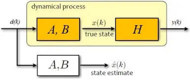
Figure 2.1: system representation by means of block diagrams.
then following that,
y(t) = HeAc (t−t0)x(t0) + t ∫
t0
HeAc (t−ξ)Bcd(ξ)dξ+Dd(t) (2.15)
The general system representation in state space form and based on block dia-grams is shown in figure 2.1.
2.3 Discrete time state-space representation
Physical quantities change continuously with time since systems in real word are characterized by a continuous-time dynamics. So what happens is that sensors generate analog acquisition continuously, but computers handle with the digital sampled signal and as a consequence state estimation and control algorithms are usually implemented by means of digital electronic (Simon, 1990). In general, a continuous time invariant system can be represented by a sampled one, as follows
x(t) = eAc (t−t0)x(t0) + t ∫
t0
eAc (t−ξ)Bcd(ξ)dξ (2.16)
Consider the discrete sampling interval∆tand substitute t0=k∆tand t = (k + 1)∆t into the above continuous solution,
x [(k + 1)∆t] = eAc∆tx(k∆t) +
(k +1)∫ ∆t
k∆t
eAc [(k +1)∆t−ξ]Bcd(ξ)dξ (2.17)
Then with the final change of variables−τ = (k + 1)∆t−ξand with some simplifi-cations one gets,
x (k + 1) = eAc∆tx(k∆t) + ∆t ∫
0
and finally, posed Ad =eAc (∆t), the solution in discrete time writes
x (k + 1) = Adx(k ) + ∆t ∫
0
e−AcτBcd(τ)dτ (2.19)
and the general form
x(k + 1) = Adx(k ) + Bdd(k ) (2.20)
It is evident that the integration in Eq. 2.19 depends on the inter-sample behavior of the input d(k ). Some assumption must be done about d(k ) and the parametrization for the inter sample behavior of the input can be expressed as (Bernal, 2007),
d(τ) =f0(τ)d(k ) + f1(τ)d(k + 1) (2.21)
where f0(τ) and f1(τ)are arbitrary basis function defined over the time step and with origin at the beginning of each time step. In general a finite dimensional input can be expressed in the inter-sample as follows,
d(τ) = ∑
alljs
fj(τ)dk +j (2.22)
Since the true analog input does not generally belong to the class that fits the discrete time state space model, for any duplet{f0,f1}, a residual exists between the true analog input and the sampled-based reconstruction. Substituting Eq. 2.21 into the integral in Eq. 2.19, the generic form of the discrete state space equation is expressed as (Hanselman, 1987)
x(k + 1) = Adx(k ) + ∑ all js
Bjd(k + j) (2.23)
where
Bj =Ad ∆t ∫
0
e−AcτBcfj(τ)dτ, for j = 0, 1 (2.24)
Table 2.1: Closed form of the state matrices as function of the discrete assumptions on the input.
Inter sample assumption B0 B1
Zero Order Hold (A −I)Ac−1Bc 0
First Order Hold (A −I)Ac−1Bc−B1 (A−Ac∆t−I)Ac−2Bc/∆t
as,
Ac = log(Ad )
∆t (2.25)
Bc = (T0+AdT1)−1Bd (2.26)
Cc =Cd (2.27)
Dc =Dd−CcT1Bc (2.28)
where
Tj=Ad ∫ ∆t
0 e −Acτf
j(τ)dτ (2.29)
2.3.1 Zero order hold
For the Zero Order Hold (ZOH) the assumption is {f0,f1} = {1, 0}, so j = 0. The continuous signal is sampled and holds at a certain value for all the intervals, becoming a stepwise as shown in figure 2.2. Let’s assume,
d(τ) =f0(τ)d(k ) (2.30)
Let’ s define Bd, assuming that t0= 0,then,
t ∫
0
Figure 2.2: discrete and continuous signal.
= t ∫
0
eAc (t−τ)Bcf0(τ)d(k )dτ= (2.32)
= t ∫
0
eAc (t−τ)Bc1d(k )dτ = (2.33)
=−AdAc−1e−AcτBc∆ t
0 d(k ) = (2.34)
=−AdAc−1 (
Ad−1−I )
Bcd(k ) = (2.35)
=Ac−1(Ad−I)Bcd(k ) (2.36)
Comparing Eqs. 2.19 and 2.20, it is evident that the ZOH solution is valid for for Bd =Ac−1(Ad−I)Bc. In addition remembering Eq. 2.24 we define that Bd = B0 and B1= 0.
2.3.2 First order hold
For the First Order Hold (FOH) the assumption is{f0,f1} = {1−τ /∆t,τ /∆t}. Let’s assume,
This parameterization is not widely used in identification theory but is likely to be more accurate than the ZOH assuming that in this case causality is not an issue, (Bernal, 2007). The state space system becomes
x(k + 1) = Adx(k ) + B0d(k ) + B1d(k + 1) (2.38)
y(k ) = Hdx(k ) + Ddd(k ) (2.39)
The above-formulation is not in a standard discrete time state-space form due to the presence of the term d(k + 1). However, it is possible to convert it in standard form using the following transformation introduced by Hanselman (1987):
x(k ) = z(k ) + ∑ all js
j ∑
i=1
Adj−iBjdk +i−1 (2.40)
and
z(k + 1) = Adz(k ) + ∑
all js AdjBj
d(k ) (2.41)
y(k ) = Ccz(k ) + Cc ∑
all js j ∑
i=1
Adj−1Bjd(k + i−j) + Dcd(k ) (2.42)
In detail, for the FOH discretization,
x(k ) = z(k ) + B1d(k ) (2.43)
and as a consequence,
x(k + 1) = z(k + 1) + B1d(k + 1) (2.44)
That yields,
z(k + 1) + B1d(k + 1) =
z(k + 1) = Adz(k ) + AdB1d(k ) + B0d(k ) = Adz(k ) +[AdB1+B0]d(k ) (2.46)
and
y(k + 1) = Hd[z(k ) + B1d(k )]+Ddd(k ) = Hdz(k ) +[HdB1+Dd]d(k ) (2.47)
Finally,
z(k + 1) = Adz(k ) +[AdB1+B0]d(k ) = A2z(k ) + B2d(k ) (2.48)
and
y(k + 1) = Hdz(k ) +[HdB1+Dd]d(k ) = H2z(k ) + D2d(k ) (2.49)
since
A2=Ad (2.50)
B2=AdB1+B0 (2.51)
H2=Hd (2.52)
D2=H2B1+Dc (2.53)
Let’s now define B2, assuming that t0 = 0and knowing the solution in continuous time,
x(t) = eAc tx(0) + t ∫
0
eAc (t−τ)Bcd(τ)dτ (2.54)
The input is sampled with a FOH:
d(τ) =d(k ) + τ
Substituting the input above into the forced part of the solution
t ∫
0
eAc (t−τ)Bcd(τ)dτ= t ∫
0
eAc (t−τ)Bc(f0(τ)d(k ) + f1(τ)d(k + 1) )
dτ (2.56)
Then we need to solve the following three integrals: ∆t
∫
0
eAc (t−τ)Bcd(τ)dτ= (2.57)
= ∆t ∫
0
eAc (t−τ)Bcd(k )dτ− ∆t ∫
0
eAc (t−τ)Bc τ
∆td(k )dτ+ ∆t ∫
0
eAc (t−τ)Bc τ
∆td(k + 1)dτ
(2.58)
Remembering that Bj = Ad ∆t ∫
0
e−AcτBcfj(τ)dτ, j = 0, 1and that B0 and B1 are
the two terms needed to find B2:
B0= ∆t ∫
0
eAc (∆t−τ)Bcf0(τ)dτ =
= ∆t ∫
0
eAc (∆t−τ)Bcd(k )dτ− ∆t ∫
0
eAc (∆t−τ)Bc τ
∆td(k )dτ (2.59)
B1= ∆t ∫
0
eAc (∆t−τ)Bcf1(τ)dτ = ∆t ∫
0
eAc (∆t−τ)Bc τ
∆td(k + 1)dτ (2.60)
It is possible to show that the solution for this integral results,
Ad(I1− I2 ∆t)d(k ) +
Ad
∆tI2d(k + 1) (2.61)
where
I1=Ac−1 [
Ad−1−I ]
Bc (2.62)
I2= [
−Ac−1Ad−1Bc∆t−Ac−2(Ad−1−I)Bc ]
2.4 Observability, reconstructability and detectability
The observability (and also the recontructability and detectability) of a system is a basic concept in the estimation and control theory (Simon, 1990). A system is observable if the current state can be determined in a finite amount of time steps using both the information contained in outputs y(t) and inputs d(t). Since we use also the outputs in order to find the current state, we must be sure that the current state can be distinguishable from another one. The pair of states x1 ̸= x2 ∈R2n is called indistinguishable from the output y(·) if for any input sequence d(·) the following applies,
y(k ; x1,d(·)) =y(k ; x2,d(·)),∀k ≥0 (2.64)
So the system is called completely observable if no pair of states are indistinguish-able from the output. The issue related to the observability process consists in determining the initial state x(k0)through observations of both the inputs d(k ) and the outputs y(k ) of the actual system, for k ≥k0.Let’ s consider the following LTI system in discrete time,
x(k + 1) = Adx(k ) + Bdd(k ) y(k ) = Hdx(k ) + Ddd(k )
,x(0) = 0 (x∈R2n,d∈Rr,y∈Rm) (2.65)
with output:
y(k ; x0,d(·)) =HdAdkx0+ k∑−1
j=0
HdAdjBdd(k−1−j) + Ddd(k ) (2.66)
The problem of reconstructing the initial condition from m output measurements is outlined in the following. The output recurrence is
y(0) = Hdx0+Ddd(0)
y(1) = HdAdx0+HdBdd(0) + Ddd(1) ..
.
y(N−1) =HdAdN−1x0+∑j=1N−2HdAdjBdd(N−2−j) + Ddd(N−1)
and we define YY =
y(0)−Ddd(0) y(1)−HdBdd(0)−Ddd(1)
.. . y(N−1)−∑N−2
j=1 HdA j
dBdd(N−2−j) + Ddd(N−1) (2.68) and Θ= Hd HdAd
.. . HdAN−1
(2.69)
So, the initial state x0is determined by solving the linear system
YY =Θx0 (2.70)
where the matrix Θ ∈ RNm×2n is the observability matrix of the system. With regard eq. 2.70,
• the solution is unique ifrank(Θ) = 2n;
• there exist infinite solutions if rank(Θ) < 2n; in this case, all solutions are given by x0+ker(Θ), where x0is any particular solution of the system.
Then, assuming that the solution is unique and knowing the initial condition x0and the inputs, the current state for any time instant k can be easily determined,
x(k ) = Adkx0+ k∑−1
i=0
AdiBdd(k−1−i) (2.71)
In order to find the initial state, we use the Rouch-Capelli theorem and as a conse-quence the system in 2.70 has a solution if
rank(Θ) =rank([ΘYY ]) (2.72)
matrixΘ, that means on the couple{Ad,Hd}. So the couple{Ad,Hd}is observable if rank Hd HdAd
.. . HdAd2n−1
= 2n (2.73)
We are interested in the kernel since in generalker(Θ)is the set of statesx ∈R2n that are indistinguishable from the origin for any input sequence d(·), which means that
y(k ; x, d(·)) =y(k ; 0, d(·)),∀k ≥0 (2.74) A system is observable if and only if there are no states that are indistinguishable from the origin x = 0 and this happens whenker(Θ) ={0}or, in other words, when rank(Θ) = 2n. A linear system x(k + 1) = Adx(k ) + Bdd(k )is called reconstructable in ksteps if, for each initial condition x0, x(k ) is uniquely determined by{d(j), y(j)}kj=0−1. A system reconstructable in N steps in completely reconstructable. Finally, the lin-ear system is detectable if it is reconstructable asymptotically for t→ ∞. It is useful to investigate the observability property since a system is in general endowed with sensors that allow to measure only a part of some state variables or their linear combination. The set of the measured variable form the set of the system outputs y(·)but there is a lack of knowledge about the dynamic field induced by a general load since the number of sensors is limited. Using the observability property of the LTI system, it is however possible to estimate the state of the system ˆx(k ) with the so called asymptotic state estimator, starting from the measurement of both the input d(·)and the output y(·), with a estimate error the asymptotically goes to zero,
lim
t→∞∥x(t)−x(t)ˆ ∥= 0 (2.75)
2.4.1 The initial condition issue
The structure of the open loop estimator is nothing else than a “copy” of the dynamic equations of real system which uses both the input d(t) and the model of the system, as shown in figure 2.3. Of course initial conditions are not known, so the output of the simulated system is biased by the error due to the lack of knowledge on initial conditions. The equations for this open loop estimator write,
Figure 2.3: Open loop state estimator.
ˆ
x(k + 1) = Adx(k ) + Bˆ dd(k ) (2.76)
The estimate error result to be
e(k ) = x(k )−x(k )ˆ (2.77)
and the dynamics of the estimate error
e(k +1) = x(k +1)−x(k +1) = Aˆ dx(k )+Bdd(k )−Adx(k )ˆ −Bdd(k ) = Ad(x(k )−x(k )) = Aˆ de(k ) (2.78)
The evolution with an initial condition e(0) = x(0)−x(0)ˆ results
e(k ) = e(0)Ad (2.79)
2.4.2 Closed loop asymptotic estimator
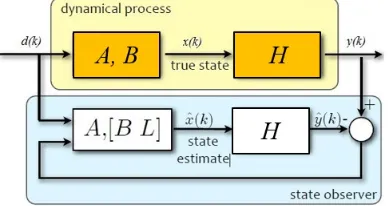
The idea behind the closed loop asymptotic estimator is to feed back the esti-mation error using the available measurements, i.e. the outputs y(t), through an appropriate gain used to change the asymptotic behavior of the estimator (Juang and Phan, 2001; Kailath, 1990). This is shown schematically in figure 2.4. The
Figure 2.4: closed loop asymptotic estimator.
closed loop asymptotic estimator uses all available information. Indeed, through an appropriate choice of the feedback gain matrix L , it is possible to control the convergence rate of the estimate error. The equation of the estimator in closed loop reads,
ˆ
x(k +1) = Adx(k )+Bˆ dd(k )+L [y(k )−Hdx(k )] = (Aˆ d−LHd) ˆx(k )+Ly(k )+Bdd(k ) (2.80) The initial state x(0) is unknown, so one uses an initial random value on the initial state estimate ˆx(0). The dynamic of the error estimate writes,
e(k + 1) = x(k + 1)−x(k + 1) =ˆ (2.81)
=Adx(k ) + Bdd(k )−Adx(k )ˆ −Bdd(k )−L [y(k )−Hdx(k )] =ˆ =Adx(k )−Adx(k )ˆ −LHdx(k ) + LHdx(k ) =ˆ
= (Ad−LHd)(x(k )−x(k )) = (Aˆ d−LHd)e(k )
convergence rate can be modulated by choosing the magnitude of the real part of the eigenvalues through the matrix L .
2.5 Dynamic response and Markov parameters
For discrete time model, the dynamic response to a general input is already built into the model. We simply need to compute the state at each time step,
x(1) = Adx(0) + Bdd(0) (2.82)
x(2) = Adx(1) + Bdd(1) = Ad2x(0) + AdBdu(0) + Bdu(1) (2.83)
x(3) = Adx(2) + Bdd(2) = Ad3x(0) + Ad2Bdu(0) + AdBdu(1) + Bdu(2) (2.84)
and so on. Eventually,
x(k ) = Adkx0+ k∑−1
i=0
AdiBdd(k−1−i) (2.85)
and the corresponding output is
y(k ) = HdAdkx0+ k∑−1
i=0
HdAdiBdd(k−1−i) + Ddd(k ) (2.86)
The output equation can be rearranged in order to highlight the Markov parame-ters Yk; in fact, the outputs are the result of the convolution between the Markov parameters and the input load.
y(k ) = HdAdkx0+ [
Dd HdBd HdAdBd HdAd2Bd ... HdAdk−1Bd ] d(k ) d(k−1)
or y(k ) y(k−1)
... ... y(1) y(0) =
HdAdk HdAdk−1
... ... HdAd
Hd
x0+
Y0 Y1 Y2 Y3 ... Yk 0 Y0 Y1 Y2 ... ... 0 0 Y0 Y1 Y2 Y3 0 0 0 Y0 Y1 Y2 0 0 0 0 Y0 Y1
0 0 0 0 0 Y0
d(k ) d(k−1)
... ... d(1) d(0) (2.88)
For zero initial condition, the well know formulation of the impulse response holds,
y(t) = Md(t) (2.89)
We note that the solution to the same input d(k ) is not the same if we are integrat-ing the differential equation in continuous time or if we are solvintegrat-ing the difference equation in discrete time. In discrete time, the response is due to the discretized version of d(k ).
2.6 LQR and LQG controller
In this chapter we introduce the basic equations of the Optimal Linear Quadratic Regulator (LQR) in continuous and discrete time and finite/infinite horizon.
2.6.1 LQR in continuous time and finite/infinite horizon
Assuming the linear system in continuous time
˙
x(t) = Acx(t) + Bcu(t) (2.90)
Let’s start using a finite time horizon; the objective is to minimize the following quadratic cost function within the time interval [t0, ...,t1],
J = x(t1)TMx(t1) + ∫ t1
t0
(x(t)TQx(t) + u(t)TRu(t))dt (2.91)
The control law results to be,
u(t) =−KLQR(t)x(t) (2.92)
where KLQR(t) = R−1BcTP(t)and P(t) is the solution of the Riccati differential equa-tion in continuous time
Let’s now take the infinite time horizon; the objective now is to minimize the follow-ing quadratic cost function within the time interval [t0, ...,∞],
J = ∫ t∞
t0
(x(t)TQx(t) + u(t)TRu(t))dt (2.94)
The control law results to be,
u(t) =−KLQR(t)x(t) (2.95)
where KLQR(t) = R−1BcTP∞and P∞is the solution of the Riccati differential equa-tion in continuous time
0 =AcTP∞+P∞Ac −P∞BcR−1BcTP∞+Q (2.96) 2.6.2 LQR in discrete time and finite/infinite horizon
Assuming the linear system in discrete time
x(k + 1) = Adx(k ) + Bdu(k ) (2.97)
Let’s start using a finite time horizon; the objective is to minimize the following quadratic cost function within the time interval [k0, ...,k1],
J = k1 ∑
i=k0
(x(k )TQx(k ) + u(k )TRu(k )) (2.98)
The control law results to be,
u(k ) =−KLQR(k )x(k ) (2.99)
where KLQR(k ) = (RT+BdTP(k )Bd)−1BdTP(k )Ad and P(k−1)is the solution of the Riccati algebraic equation in discrete time
P(k −1) =AdT(P(k )−P(K )Bd(R + BdTP(k )Bd)−1BdTP(k ))Ad+Q (2.100) Let’s now take the infinite time horizon; the objective now is to minimize the follow-ing quadratic cost function within the time interval [k0, ...,∞],
J = ∞ ∑
i=k0
The control law results to be,
u(k ) =−KLQR(k )x(k ) (2.102)
where KLQR(k ) = (RT+BdTP∞B)−1BdTP∞Adand P∞is the solution of the Riccati algebraic equation in discrete time
P∞=AdT(P∞−P∞Bd(R + BdTBd)−1BdT)Ad+Q (2.103) 2.7 Modal domain
The dynamic behavior of structures can be settled by only few vibrational modes (Ewins, 2000). It can be useful to project the problem into the modal domain. Start-ing from the equation of motion in continuous time,
M ¨u(t) + C ˙u(t) + Ku(t) = Sd(t) (2.104)
The change of coordinates writes,
u(t) =Φq(t) (2.105)
The introduction of modal coordinates and the pre-multiplication byΦT, yields
ΦTMΦu(t) +¨ ΦTCΦu(t) +˙ ΦTKΦu(t) =ΦTSd(t) (2.106)
and assuming proportional damping, the decoupled system becomes
I ¨q(t) +Γq(t) +˙ Ω2q(t) =ΦTSd(t) (2.107)
where the diagonal matrix Ω ∈ Rnxn collects the n eigenfrequencies. The state space system in modal domain givenζ= q(t)
˙
q(t), results
˙ ζ(t) =
0 I
−Ω2 −Γ ζ(t) +
0
ΦTS
d(t) (2.108)
or
˙
ζ(t) = Amζ(t) + Bmd(t) (2.109)
with Am∈R2nx2n, Bm∈R2nxr,ζ∈R2nandd(t)∈Rr. With regard to the measure-ment equation, displacemeasure-ment, velocity and acceleration measuremeasure-ment can easily be projected in the modal domain
y(t) = Rvu(t) = R˙ vΦq(t)˙ (2.111)
y(t) = Rau(t) = R¨ aΦq(t)¨ (2.112)
with Rd, Rv and Ra ∈Rnxnallowable to selecting for the real position of displace-ment, velocity and acceleration measurements, respectively. In turn, acceleration can be written as,
I ¨q(t) =−Γq(t)˙ −Ω2q(t) +ΦTSd(t) (2.113) and substituting (in the case of acceleration data),
y(t) =−RaΦΓq(t)˙ −RaΦΩ2q(t) + RaΦΦTSd(t) (2.114) or
y(t) = [
−RaΦΩ2 −RaΦΓ ] q(t) ˙ q(t) + [
RaΦΦTS ]
d(t) (2.115)
Collecting different types of measurements, the output equation write
y(t) = u(t) ˙ u(t) ¨ u(t) =
RdΦ 0
0 RvΦ
−RaΦΩ2 −RaΦΓ ζ(t) +
0 0 RaΦΦTS
d(t) (2.116)
or easily
y(t) = Hmζ(t) + Dmd(t) (2.117)
with Hm∈Rmx2n, Dm∈Rmxr,ζ∈R2nand d(t)∈Rr. 2.8 Model reduction
It is often necessary to cut off the problem dimension because of computa-tional issues by means of a model reduction. When the reduction is performed, the dynamics of the system is represented by a reduced number N of modal coor-dinates. ζr(t)∈R2N is the modal state vector and the state vector is just a linear combination of N modes where
ΦT
r MΦru(t) +¨ ΦTr CΦru(t) +˙ ΦTr KΦru(t) =ΦΦTSd(t) (2.119)
The expression for modal acceleration becomes
I ¨qr(t) +Γrq˙r(t) +Ω2rqr(t) =ΦTr Sd(t) (2.120)
and the modal reduced model in state space yields,
˙
ζr(t) = Am,rζr(t) + Bm,rd(t) (2.121)
with Am∈R2Nx2N, Bm∈R2Nxr,ζ∈R2N and d(t)∈Rr. With regard to the output equation, y(t) = u(t) ˙ u(t) ¨ u(t) =
RdΦr 0 0 RvΦr
−RaΦrΩ2r −RaΦrΓr ζr(t) +
0 0 RaΦrΦTr S
d(t) (2.122)
or easily
y(t) = Hm,rζ(t)r +Dm,rd(t) (2.123)
CHAPTER
3
THE KALMAN FILTER THEORY FOR INPUT AND STATE
ESTIMATION
3.1 Introduction
Theory of state estimations stems from the necessity of estimating instanta-neous state of a linear dynamic system by means of the output measurements which are both linearly related to the state and corrupted by noise. The state esti-mation arises from the fact that the control of complex dynamic systems need the knowledge of the motion field, but the availability of measurement points is limited and it not possible to measure all wanted variables.
chapter the basic concepts about the linear Kalman filter for state and input identi-fication are introduced. Then the Chapter the focus shifts on the non-linear version of the filter and on its utilization as state and parameter estimator for non-linear systems.
3.2 The Kalman Filter
The model considered by the KF has uncertainties related to:
• unknown inputs;
• discrepancies between the real system and the analytical model;
• unknown initial conditions.
The KF is a recursive data processing algorithm, which provides the optimal state estimate of the system that is subjected to stationary stochastic disturbances with known covariances. More precisely, the Filter computes the conditional mean and covariance of the probability distribution of the state of the linear stochastic system with noises defined in the following. Let’s consider the following time invariant linear system in discrete time,
xk =Axk−1+Buk−1+Gwk−1 (3.1)
yk =Hxk +vk (3.2)
where the system matrix are A ∈ R2nx2n, B ∈R2nxr, H ∈Rmx2n and G ∈ R2n. xk ∈ R2n is the state vector, dk ∈ Rr is the deterministic input and yk ∈ Rm is the available measurement vector. The sequence wk ∈ R2n is the known distur-bance also known as process noise and vk ∈Rmis the measurement noise. It is assumed that the noises are Gaussian stationary white noise with zero mean and known covariance matrices (although these assumptions are quite distant from reality),
E(xk) = ˆx0
E((x0−xˆ0)(x0−xˆ0)T) =P0
E(wk) = 0 (3.4)
E(vk) = 0 (3.5)
and
E(wkwjT) =Qδkj (3.6)
E(vkvjT) =QRδkj (3.7)
E(wkvjT) = 0 (3.8)
whereδkjis the Kronecker Delta. In addition, the state is uncorrelated with respect to the noises, i. e.
E(xkwjT) = 0 (3.9)
E(xkvjT) = 0 (3.10)
3.2.1 The state estimator
A linear estimator for a LTI is,
ˆ
xk +1=F ˆxk +Zdk +Lkyk (3.11)
where ˆxk is the estimate of xk and Lk is the observer gain. Let’s define the error between the real state and its estimate,
ek =xk −xˆk (3.12)
and substituting for the time station k + 1 Eq. 3.1 and Eq. 3.2 into Eq. 3.12, it holds,
replacing xk with ˆxk −ek,
ek +1= (A−LkHk)( ˆxk −ek) + (B−Z )dk +Gwk +F ˆxk −Lkvk (3.14) reordering
ek +1= (A−LkHk)ek + (B−Z )dk +Gwk + (A −LkH−F) ˆxk −Lkvk (3.15) and taking the expected value of Eq. 3.15 and knowing Eqs. 3.4 and 3.5, one finally obtains,
E(ek +1) = (A−LkHk)E(ek) + (B−Z )E(dk) + (A−LkH−F)E( ˆxk) (3.16) Since the expected values of the state estimate and of the input are not necessarily zero and since we want that the expected value of the error is zero, it is necessary that,
Z = B (3.17)
and
F = A−LkH (3.18)
So the error in the time station k + 1 is a function of the error and the noises at the previous step,
ek +1= (A−LkHk)ek +Gwk −Lkvk (3.19) and its expected value
E(ek +1) = (A−LkHk)E(ek) (3.20)
Hence, it is necessary that
limk→∞E(ek +1) = 0 (3.21)
3.2.2 Innovation form of the Filter
Let’s define now the error in the state before and after the measurement update reads,
e−k =xk −xˆk− (3.22)
e+k =xk −xˆk+ (3.23)
where ˆxk−is the a priori estimate and ˆxk+is the a posteriori estimate. The covariance of the estimation error before and after the update
Pk−=E[e−k e−kT] =E[(xk −xˆk−)(xk −xˆk−)T] (3.24)
Pk+ =E[ek+ek+T] =E[(xk −xˆk+)(xk −xˆk+)T] (3.25) We postulate the existence of the state estimate before and after that information from measurements became available, so
ˆ
xk−=A ˆxk+−1+Bdk−1 (3.26)
ˆ
xk+= ˆxk−+Kk(yk −H ˆxk−) (3.27) The first step represented by Eq. 3.26 identifies the prediction step of the Filter, while in the second step, an update of the current a priori state estimate occurs since the first estimate is corrected by the measurement vector that now is avail-able. The a priori estimate error writes
e−k =Axk−1+Bdk−1+Gwk−1−A ˆxk+−1−Bdk−1 (3.28) which reduces to
and its the covariance results
Pk−=APk+−1AT +GQGT (3.30)
Then, let’s take the a posteriori state estimate and use the substitution of Eq. 3.2,
ˆ
xk+= ˆxk−+Kk(Hxk +vk −H ˆxk−) (3.31) substituting Eq. 3.23 into Eq. 3.31, yields
xk −ek+=xk −e−k +Kk(Hxk +vk −H ˆxk−) (3.32) and reorganizing
ek+=e−k −Kk(Hek−+vk) (3.33)
So the second important result is the covariance of the a posteriori estimation error
Pk+=E[ek+ek+T] =E[(ek−−Kk(Hek−+vk))(e−k −Kk(Hek−+vk))T] (3.34)
Pk+=Pk−−Pk−HTKk +KkRKkT −KkHPk−−KkHPk−HTKkT (3.35) The goal is to find the gain Kkthat minimizes this a posteriori covariance. Taking the derivative of Eq. 3.35 with respect to Kk, gives
Kk =Pk−HT(HPk−HT+R)−1 (3.36)
finally after obtaining the gain, we can reformulate the expression for the a poste-riori covariance,
Pk+= (I−KkH)Pk− (3.37)
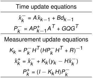
The filter steps are summarized in table 3.1 3.2.3 The steady state form of the Filter
Table 3.1: Discrete-Time filter equation.
Time update equations
ˆ
xk−=A ˆxk−1+Bdk−1 Pk−=APk+−1AT+GQGT Measurement update equations
Kk =Pk−HT(HPk−HT+R)−1 ˆ
xk+= ˆxk−+Kk(yk −H ˆxk−) Pk+= (I−KkH)Pk−
in time since once the transient response due to the error in the initial estimate ˆx0 is dissipated, the state estimation error become stationary and consequently the error covariance converges at the steady state value. The steady state value is available from the solution of the discrete algebraic Riccati Equation
P = APAT−APHT(HPH + R)−1HPAT+GQGT (3.38) This equation can be solved under conditions of uniqueness:
• A is stable
• the pair (A , H) is observable
• the pair (A , GQGT)is controllable
• R>0
• GQGT >0.
Similarly the gain results to be
K = PHT(HPHT+R)−1 (3.39)
3.2.4 The Kalman-Bucy filter
The Kalman-Bucy filter is the continuous form of the filter. The continuous-time random process x(t) and the observations are given by
˙
y(t) = Hc(t)x(t) + v(t) (3.41)
with, as usual
E[w(t)vT(τ)] = 0∀t,τ≥0 (3.42)
E[w(t)wT(τ)] =Q(t)δ(t−τ) (3.43)
E[v(t)vT(τ)] =R(t)δ(t−τ) (3.44)
E[x0] = ¯x0 E[(x−x¯0)(x−x¯0)T] =P0 (3.45)
E[x0wT(t)] = 0 E[x0vt(t)] = 0 (3.46)
The observer
˙ˆx(t) = Ac(t) ˆx(t) + Bc(t)d(t) + K (t)[y(t)−Hc(t) ˆx(t)] (3.47) whilst the matrix Riccati differential equation to be solved reads,
˙
P(t) = Ac(t)P(t) + P(t)AcT(t)−P(t)HcT(t)R−1(t)Hc(t)P(t) + Q(t) (3.48) and the gain in continuous time results,
K (t) = P(t)HcT(t)R−1(t) (3.49)
3.3 The Kalman Filter for input identification
3.3.1 RLS approach
Tuan et al. (1996) and Tuan et al. (1997) show a Kalman-like observer joined with a Recursive Least Square (RLS) approach in order solve a typical Inverse Heat Conduction Problem (IHCP). In such a problem, it is desired to estimate the unknowns of a thermal system (heat fluxes or heat sources) providing temperature measurements in the interior of the body. In the papers, the goal is to estimate the thermal unknowns by using temperature measurements in order to estimate both the states and the operating load. The algorithm consists in two parts: the Kalman filter and the Recursive Least Square weighted by a forgetting factor.
Figure 3.1: state and input observer layout.
Table 3.2: RLS algorithm Step Equation State xk +1 = Ax k + Bd k + wk Measurements yk = Hx + vk Initialization
ˆxk−
1 | k − 1 ,P k − 1 | k − 1 ,d k − 1 ,P b ,k − 1 Optimal Kalman obser v er A pr ior i state estimate
ˆxk|
k
−
1
=
A
ˆxk−
1 | k − 1 + B
ˆ dk−
1 A pr ior i error co v ar iance Pk | k − 1 = AP k − 1 | k − 1 A T + BQB T Inno v ation co v ar iance Sk = HP k | k − 1 AH T + R Kalman gain Ka ,k = Pk | k − 1 H T S − 1 k Inno v ation ˆyk = yk − H
ˆxk|
k − 1 A poster ior i state estimate
ˆxk|
k
=
ˆxk|
k − 1 − Ka ,k A poster ior i error co v ar iance Pk | k = [I − Ka ,k H ]P k | k − 1 Recursiv e least square algor ithm Sensitivity matr ices Mk = [I − Ka ,k H ][ AM k − 1 + I] Bs ,k = H [AM k − 1 + I] B Input estimate gain Kb ,k = γ − 1 P b ,k − 1 B
T s,k
[B
T s,k
γ − 1 P b ,k − 1 B
T s,k Sk − 1 ] − 1 Error co v ar iance Pb ,k = [I − Kb ,k Bs ,k ] γ − 1 P b ,k − 1 Input estimate
ˆ dk
=
ˆ dk−
1 + Kb ,k [ˆyk − Bs ,k
ˆ dk−
1
The Kalman filter generates the recursive relation between the observed value of the innovation without knowledge of the input and the theoretical residual as-suming that the input is obtained. In this relationship there is a deterministic bias due to the unknown input and a random bias due to the process and measure-ment noise. In the meanwhile, the RLS algorithm uses the residual to extract the estimated deterministic input.The adaptive procedure can be implemented on-line. The starting point is the discrete time invariant system and the complete observer layout is in figure 3.1. In this procedure, the Kalman filter acts as a ”bias free“ estimator and the RLS function as a ”bias“ estimator. The input gain minimizes the difference between actual and estimated loads; the forgetting factor weights the error on the input estimate by giving less importance to the oldest samples. De-tails of the algorithm are shown in figures 3.2 and 3.3. In Table 3.2 is reported the
Figure 3.3: the RLS observer.
whole algorithm. The application of the Kalman Filter with a recursive estimator is also used in Liu et al. (2000) in order to determine the input force of a cantilever plate.
3.3.2 Minimum-Variance Unbiased input and state estimation algorithms
Unbiased (MVU) input and state estimation. The recursive filter is used on linear discrete-time system in order to jointly estimate the state and the input. The input estimate is obtained through a least square procedure and the extended state es-timate is obtained from a standard Kalman approach. Results are coherent with both the Kitanidis (1987) and Darouach and Zasadzinski (1997) state estimation, and with the input estimation of Hsieh (2000). Consider the Linear Time Invariant (LTI) discrete-time system,
xk +1=Axk +Bdk +wk (3.50)
yk =Hxk +vk (3.51)
where xk ∈ R2n is the state vector, dk ∈ Rr is the unknown input and yk ∈Rm is the measurement vector. The process noise wk ∈ R2n and the measurement noise vk ∈Rmare assumed to be mutually uncorrelated, zero-mean, white random signals with covariance matrices Qk and Rk.The input has unknown model and no a priori assumption is made on it. The relevant pseudo-code results to be,
• Initialization: x0= ˆxk−1|k−1,P0=Pk−1|k−1.
• Input estimation:
1. ˆxk|k−1=A ˆxk−1|k−1is biased by the unknown input
2. Pk|k−1=APk−1|k−1AT+Q
3. ˜Rk =HPk−1|k−1AHT+R
4. Mk = (FkTR˜−1
k Fk)FkTR˜k−1, where Fk =HB 5. d−ˆ 1
k = Mk(yk −H ˆxk|k−1)is the MVU estimate of the unknown input given the innovation yk −H ˆxk|k−1.
• State estimation:
State update
1. ˆxk∗|k = ˆxk|k−1+B ˆdk−1is the unbiased state estimate of xk
2. Kk =Pk|k−1HTR˜−1
3. Pk∗|k = (In−BMkH)Pk|k−1(In−BMkH)T +BMkRMkTBT. Measurement update
1. ˆxk|k = ˆxk∗|k +Kk(yk −H ˆxk∗|k)is the MVU estimator of xk 2. Sk∗=−BMkR
3. Pk|k =Pk∗|k −Kk(Pk∗|kHT+Sk∗)T.
Consider now the Linear Time Invariant (LTI) discrete-time system:
xk +1=Axk +Bdk +wk (3.52)
yk =Hxk +Ddk +vk (3.53)
• Initialization: x0= ˆxk|k−1,P0x =Pkx|k−1.
• Input estimation:
1. ˜Rk =HPk|k−1AHT+R
2. Pkd = (D ˜Rk−1DT)−1
3. Mk =PkdDTR˜−1 k
4. ˆdk =Mk(yk−H ˆxk|k−1)is the MVU estimate of the unknown input given the innovation yk −H ˆxk|k−1.
• State estimation:
Measurement update
1. Kk =Pkx|k−HTR˜k−1
2. ˆxk|k = ˆxk|k−1+Kk(yk −H ˆxk|k−1−D ˆdk) 3. Pkx|k =Pkx|k−1−Kk( ˜Rk −DPkdDT)KkT 4. Pkxd = (Pkdx)T =−KkDPkd
Time update
1. ˆxk +1|k =A ˆxk|k +B ˆdk
2. Pk +1x |k = [
A B ]
Pkx|k P xd k
Pkdx Pkd AT
BT +Q
Lastly, time update and measurement update equations are the same used in the Kalman filter with the significant difference that the unknown input is obtained from a least square estimation. The input estimate relies on the state covariance matrix and in turn the state estimate depends from the innovation taking into account for the input estimate.
3.3.3 The steady state observer method