Symptotics: a framework for estimating the scalability
of real-world wireless networks
Ram Ramanathan1•Ertugrul Ciftcioglu2,5•Abhishek Samanta3,4• Rahul Urgaonkar1,6•Tom La Porta2
ÓSpringer Science+Business Media New York 2016
Abstract We present a framework for non-asymptotic analysis of real-world multi-hop wireless networks that captures protocol overhead, congestion bottlenecks, traffic heterogeneity and other real-world concerns. The frame-work introduces the concept of symptotic scalability to determine the number of nodes to which a network scales, and a metric calledchange impact valuefor comparing the
impact of underlying system parameters on network scal-ability. A key idea is to divide analysis into generic and specific parts connected via a signature—a set of govern-ing parameters of a network scenario—such that analyzgovern-ing a new network scenario reduces mainly to identifying its signature. Using this framework, we present the first closed-form symptotic scalability expressions for line, grid, clique, randomized grid and mobile topologies. We model both TDMA and 802.11, as well as unicast and broadcast traffic. We compare the analysis with discrete event sim-ulations and show that the model provides sufficiently accurate estimates of scalability. We show how our impact analysis methodology can be used to progressively tune network features to meet a scaling requirement. We uncover several new insights, for instance, on the limited impact of reducing routing overhead, the differential nature of flooding traffic, and the effect real-world mobility on scalability. Our work is applicable to the design and deployment of real-world multi-hop wireless networks including community mesh networks, military networks, disaster relief networks and sensor networks.
Keywords Multi-hop wireless networkNetwork designScalability Performance model
1 Introduction
The scalability of multi-hop wireless networks has been a topic of much interest over the last several years. A seminal paper by Gupta and Kumar [2] showed that the asymptotic per-node transport capacity of an arbitrary multi-hop wireless network is Hð1=pffiffiffinÞ, wheren is the number of nodes. In other words, the information carrying capacity becomes vanishingly small with increasing n. Following The views and conclusions contained in this document are those of
the authors and should not be interpreted as representing the official policies, either expressed or implied, of the Army Research Laboratory or the U.S. Government. The U.S. Government is authorized to reproduce and distribute reprints for Government purposes notwithstanding copyright notation here on.
& Ram Ramanathan [email protected] Ertugrul Ciftcioglu [email protected] Abhishek Samanta [email protected] Rahul Urgaonkar
[email protected] Tom La Porta
1 Raytheon BBN Technologies, Cambridge, MA, USA 2 Pennsylvania State University, State College, PA, USA 3 Northeastern University, Boston, MA, USA
4 Present Address: Google, Mountain View, CA, USA 5 Present Address: IBM Research, Yorktown Heights, NY,
USA
this result, there have been numerous other results char-acterizing the scalability using a similar framework but with different sets of assumptions (e.g [3–6]).
While this body of work has provided tremendous the-oretical insight, their applicability to the scalability ofreal world wireless networks in practice is limited for two reasons. First, these results are asymptotic in nature, that is, refer to the order of growth in the limit of some metric (usually transport capacity) as a function of size. In con-trast, in the real world we seek the (approximate) number of nodes beyond which a network will not work ‘‘ade-quately’’ (for some definition of ‘‘ade‘‘ade-quately’’—a topic we consider in detail in this paper). A network may be asymptotically unscalable, yet scale comfortably to the requisite number of nodes in a given deployment.1
Second, they do not consider aspects that are critical to real-world networks, such as the presence of network protocols and their overhead, the effect of congestion bottlenecks, and the diversity of traffic (e.g. unicast co-existing with broadcast). These aspects are not interesting to information theoretic analysis that focuses on scaling ‘‘laws’’. The nature of routing and medium access proto-cols,the traffic mixture and bottleneck effects, however, clearly have a significant effect on capacity and therefore need to be captured in order to suitably characterize real-world networks.
In this paper, we presentsymptotics—a framework for approximate non-asymptotic closed-form modeling of wireless network performance. Unlike asymptotic analysis that typically characterizes a network in binary terms (‘‘does it scale or not’’), symptotics seeks to provide a qualified answer (‘‘to how many nodes does it scale’’). To this end, the framework introduces the concept ofsymptotic scalability. It expresses scalability in terms of not only node capacity, but also real-world concerns including protocol overhead effects, congestion bottlenecks and multiple traffic types such as unicast and broadcast. It provides a unified approach to analytically model a suite of network scenarios without re-working the analysis for each, and a systematic way of determining the impact of changing a scenario parameter on performance. Finally, it provides closed-form models which, although harder than numerical solutions, give us insight into relationships between parameters and enable sensitivity (impact) analysis.
Our thesis is that the performance of a network scenario is dominated by a few major factors, and by focusing on those, one can obtain closed-form models with reasonable accuracy while avoiding complexity. Specifically, we
divide the model into two parts—(a) a generic equation for a class of network scenarios that captures the performance in terms of a set of major factors termed the signatureof the scenario; (b) instantiation of this equation using the specific signature of the given network scenario to derive a non-asymptotic (symptotic) closed-form expression for this network scenario. Thus, analyzing a new scenario requires doing only part (b) rather than re-working from scratch. Using the Sage mathematical software [8], we have been able to analyze new scenarios or different parameter values very quickly.
We illustrate the application of our framework by first deriving approximate symptotic scalability expressions for three static, regular topologies (line, grid, clique). For each we derive expressions with two MAC protocols (TDMA, 802.11) and two traffic types (unicast, broadcast), giving 12 models in all. A comparison with simulation results shows that despite their simplicity, our models are adequate for estimating the approximate scalability in practice, and lend support to our thesis that reasonable accuracy can be obtained with simple, approximate models. We then apply our framework to more complex topologies such as random and mobile networks, and derive closed form symptotic expressions for those scenarios.
A valuable part of the symptotic framework is a rigorous and uniform approach to impact analysis, that is, which parameters affect the overall system performance the most. As part of the framework, we introduce the concept of
change impact value (CIV) to quantify the impact of
domain parameters in a uniform way. By comparing the CIVs, we can tell, for example, if halving the offered load is better or worse for scalability than halving the routing overhead. We show how one can use CIV’s to swiftly tune a network’s features to meet a scaling requirement and estimate which parameter is critical in which conditions.
Using symptotic analysis, we have uncovered several new insights on multi-hop network performance that are difficult to discern using asymptotic analysis. We show that the impact of reducing routing overhead pales in compar-ison with that of equivalent changes in the radio rate or load (effected via compression techniques, for example) in typical scenarios. Load balancing, a relatively neglected approach, on the other hand not only increases scalability but also increases the gains from reducing overhead. The scalability behavior under flooding (network-wide broad-cast) traffic is markedly different from that under unicast traffic, for instance in its dependence on density and rela-tive performance between a randomized and regular grid. Finally, we observe that the repeated traversal mobility pattern reduces scalability by over an order of magnitude for typical parameters.
In the tradeoff between analytical accuracy and tractability, our framework makes a deliberate move 1 For example a multi-hop wireless network with directional
toward approximate, but tractable formulations. There are three reasons for this. First, analytical characterization of a real-life system and environments is inherently extremely difficult and would be near impossible without abstrac-tions. Second, from a pragmatic (vs. pedagogical) view-point, an analytical model is most useful for obtaining insights into relationships and making rough order-of-magnitude analysis—the vagaries of a wireless network render even the most painstaking analysis inaccurate in practice, and thus simple-but-approximate is better suited. Third, we recognize that the relationship between effort and accuracy is non-linear, and there exists a ‘‘knee’’ of the curve which can give us sufficient accuracy without excessive analytical effort. Our simulation validation results (detailed in Sect.5) bear testimony to the fact that such an approach can indeed bound inaccuracy to the desired level. Further, many analytical models become so abstruse in their desire to model every single detail that they lose their ability to provide insight—the very moti-vation for analysis in many cases—by being too compli-cated. The symptotics framework prioritizes simplicity by ignoring those aspects modeling which will likely not yield a commensurate benefit in accuracy. We have verified that the accuracy is still very good (see simulation results in Sect.5).
The rest of the paper is organized as follows. We begin by discussing related work in Sect.2. Section3 describes the symptotic framework, and the derivation of a ‘‘master template’’ equation. In Sect.4we illustrate the use of our framework by analyzing static, regular network scenarios. In Sect.5we compare the analytical model with simulation results for the same network scenarios using ns-2. In Sect.6 we illustrate how the framework can be extended beyond regular networks to random and mobile scenarios. Impact analysis is covered in Sect.7, after which we pre-sent some concluding remarks.
2 Related work
The scalability of wireless networks has mostly been studied along asymptotic, and information-theoretic lines—[2–6] are a representative sample. Such asymptotic analyses seek to determine the fundamental scaling law underlying a network in terms of the order-of-growth. In [2], often considered the seminal paper in this area, the authors show that the per-node transport capacity of arbi-trary wireless networks grows as Hð1ffiffi
n
pÞ indicating asymptotic un-scalability. In [3], random mobile networks are shown to scale asHð1Þ, or in other words, asymptoti-cally scalable assuming unlimited delay tolerance.
Directional antennas are shown not to help in the asymp-totic sense [4] whereas distributed MIMO [6] with some assumptions scales as Hð1Þ. In this body of work, the assessment of scalability is unqualified (e.g. ‘‘Network X does not scale’’), whereas symptotics seeks a qualified assessment (e.g. ‘‘Network X with parameter set P scales to 1000 nodes’’). Further, these works do not consider real-world aspects such as protocol overhead, bottlenecks, or traffic heterogeneity.
There has been some recent work non-asymptotic analysis [9–13], but these have focused on specific aspects such as spectrum sensing [10], latency issues [11, 13], or gateway effects in mesh networks [12], and none of them consider the effects of routing control protocols or mobility.
Analysis of specific protocols, especially 802.11, has received a lot of attention [14–16], and specific properties of OLSR [17] have been analyzed [18]. Regular networks have been analyzed in [19,20] for stability and capacity, albeit with specific focus on capacity regions [19] or impact of buffer sizes [20]. Related work for our impact analysis methodology is sensitivity analysis, which has been studied using simulation [21], and analytically using Automated Differentiation techniques in [22]. Some of these works consider real-world aspects, but focus on specific protocols or issues (e.g. delay) rather than the system as a whole, and are not focused on scalability. They also do not target closed-form expressions, which we seek due to their ability to provide insights and assist in impact analysis. Our prior works [23,24] adopt a similar analytical approach but not in depth, and do not consider randomized or mobile networks.
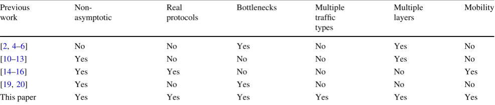
Table 1 compares this paper with a representative sample of the above works along several dimensions. This paper is the first system-level (vice individual protocols), non-asymptotic, closed-form analytical model of real-world multi-hop, possibly mobile networks that considers control protocol effects at multiple layers and non-gateway congestion bottlenecks, and accommodates impact analysis.
3 The symptotic framework
In this section, we describe the basic symptotic model, provide a formal definition for symptotic scalability, and derive a master expression that can be instantiated for various specific models in subsequent sections.
The fundamental entity for analysis in our framework is
a network scenario, which we define as a particular
attributes (e.g. rate, number of transceivers), and control mechanisms (e.g. 802.11, OLSR).
Consider a representative nodemin the network, along with its immediate neighborhood, as shown in Fig.1. We begin with a few definitions. Theavailable capacity W(m) indicates the amount of data that can be handled bym. The
demanded capacity D(m) denotes the amount of data load at m as a result of the offered traffic flows. We assume there are multiple classes ortypesof flows (e.g. web access, video etc), each of which can be one of network-wide broadcast (‘‘flooding’’) or unicast (with uniform random source destination pairs). We assume that all flows of a given type have the same load profile in terms of packet rate and size. Note that we donotassume that all traffic is the same–different flow types can have different rates and packet sizes. The blocked capacity B(m) denotes the capacity that is unusable by nodem(for example, due to contention). Theresidual capacity R(m) is the difference
WðmÞ DðmÞ BðmÞ. For node m to be able to carry demanded traffic,WðmÞ[DðmÞ þBðmÞ.
Both Dand Bmay have components stemming from several flow types, each of which may have a different ‘‘cast’’ (unicast, broadcast) and/or a different ‘‘scope’’ (e.g., a one hop ‘‘Hello’’ vs. a network wide broadcast). Data, MAC control, network control, network management control etc., each have a different combination of cast and scope and are modeled as a different component ofDand
B. Thus, there are (the same)Ttraffic components at each node, each componentj(1 j T) offers a different kind
and amount of load on the network, and DandBare the sum of different componentsj. Thus, we have,
RðmÞ ¼WðmÞ X
T
j¼1
DjðmÞ
XT
j¼1
BjðmÞ ð1Þ
Since control traffic can be thought of as a unique profile based on scope and cast, Eq. 1captures not only data but also network control such as routing updates, thereby capturing overhead effects in our framework.
For sufficiently large networks with the kinds of topologies and random traffic that we consider in this paper (see Sect.3.1), the average traffic demand on neighbors of a nodemin steady state is approximately the same as onm. Note that we donotassume that allnodes in the network have the same, or even approximately the same load. Thus,
BjðmÞ CjðmÞ DjðmÞ ð2Þ
whereCjðmÞis the number of nodes in the neighborhood
ofmthat either cause interference to, or in some other way causemto defer when they are active, thereby contributing toB(m).
We termCj , that is the number of contending nodes, as
the contention factor for component j. The contention factor CjðmÞ depends on the topology around m, on the
medium access control protocol in use, and the kind of transmission (e.g. unicast or broadcast), which in turn depends on the flow type of j. The contention factor is related to the spatial reuse achieved in a wireless network. The higher the contention factor, the lower is the spatial reuse. The total contending load is the contention factor multiplied by the average load per contending node.
Thus, from Eqs.1 and2, we have
RðmÞ WðmÞ X
T
j¼1
ð1þCjðmÞÞDjðmÞ ð3Þ
Now consider DjðmÞ. This is the contribution to m’s
demanded capacity from component j. Let Ljdenote the
offered load for a given componentj. The contribution to
DjðmÞis the traffic sourced bymplus the traffic from other
Table 1 Comparison of the Symptotic model presented in this paper with previous work on analytical capacity/scalability modeling
Previous work
Non-asymptotic
Real protocols
Bottlenecks Multiple traffic types
Multiple layers
Mobility
[2,4–6] No No Yes No Yes No
[10–13] Yes No No No Yes No
[14–16] Yes Yes No No No Yes
[19,20] Yes No Yes No No No
This paper Yes Yes Yes Yes Yes Yes
Each (i,j) entry is a Yes if paperimodels attributej, and No if it does not. Our paper is unique in that it captures a unique set of real-world concerns
D1 B1 D2 B2 Traffic 1
Traffic 2 Av
ailable(W)
Node m
Demand(D) Blocked(B) Residual(R)
sources relayed bym. We call the latter (the relayed traffic) thetransit factorofj, and denote it byj . For example, in
a 5 node line network with each node flooding one packet each, 4 packets are relayed by the central node, and so its transit factor is 4. A beacon signal sent periodically by a node has a transit factor of 0 since it is not relayed. The expected demanded capacity is then DjðmÞ ¼Lj ð1þ
jðmÞÞ.
Finally, many medium access control schemes such as CSMA/CA have non-trivialinefficiency, that is, the effec-tive rate is lower than the actual rate. Thus, the actual capacity available for multi-access communications is a fraction ofW. Denoting MAC efficiency by g, and based on the above discussion, we rewrite Eq.3 as
RðmÞ gWðmÞ X
T
j¼1
ð1þCjðmÞÞLjð1þjðmÞÞ ð4Þ
We note that the Eq.4 captures, in a unified way, both control and data flows each of which can be unicast or broadcast, the differences factored in terms of the con-tention and transit factors. Using Eq.4, we now consider the definition of symptotic scalability and the generation of a ‘‘master template’’ for symptotic analysis.
3.1 Symptotic scalability
As motivated in Sect. 1, we seek non-asymptotic scala-bility, that is, to provide an answer to a question such as ‘‘to how many nodes will my network scale’’? We begin by observing that such a question only makes sense for ex-pandable network scenarios, that is, those that have a ‘‘scale agnostic’’ specification that allows one to create a network scenario at any scale. Examples of expandable network topologies includeregulartopologies such as line, ring, grid etc., as well as irregular stationary topologies based on some probabilistic model (e.g random unit-disk graphs, scale-free networks etc.), and mobile scenarios that have an expandable mobility model (e.g. the random waypoint model).
An arbitrary network with a specific set of nodes and a specific set of links between them is not expandable because there is no ‘‘rule’’ to generate higher-sized ver-sions. Thus, the question ‘‘to how many nodes will a net-work scale’’ is well formed only for expandable netnet-works, and not for arbitrary networks. We emphasize that our use of expandable networks is a necessary outcome of the question, and not an assumption that we are making. A similar differentiation can be made with respect to traffic as well. On the other hand, note that computing the
throughput capacity of a given network is a reasonable proposition for non-expandable networks.
We consider the class of expandable networks for which the residual capacity monotonically decreases as the sizeN
increases. This class clearly includes regular networks with uniform traffic model. It also includes irregular expandable networks averaged over multiple instances, although a
particularrandom network of sizeNmay happen to have a higher residual capacity than a particular random network of sizeN1. An example of a network scenario not in this class is when the set of nodes sourcing traffic is constant (say 1). Network scenarios not in this class are arguably asymptotically scalable and so are not of interest for symptotics.
For expandable networks, there is a point at which the monotonically decreasing residual capacity transitions from positive to negative. This is the maximum number of nodes supportable, or the ‘‘symptotic’’ scalability. We formalize this notion below. First, consider static networks. Let RNðmÞ denote the residual capacity of node m in a
mobile network scenario withNnodes.
Definition 1 Thesymptotic scalabilityof a static network scenario is the number of nodesXsuch that for allNX, and for all nodesm,RNðmÞ 0, and for all N[X, there
exists a nodemb such thatRNðmbÞ\0.
We call mb a bottleneck node. As the network size is
increased, the bottleneck node is the node at which the residual capacity first becomes negative, and the size at which this happens is the symptotic scalability. When the residual capacity is positive, the bottleneck node is rate-stable, that is, the input rate is less than the service rate. A network scenario may have multiple bottlenecks, that is, nodes with equally lowest residual capacity, in which case
mb is any one of them.
We now consider mobile networks. We model mobile networks as a time-series of static network snapshots. Each snapshot is independent of the other, that is, there are no carryovers of queues from one snapshot to the next. This is a reasonable assumption in practice as typically the time scales for traffic dynamics are much smaller than those for topology changes. Each snapshot may be treated as a static network per Definition1 and assessed for symptotic scal-ability. We define the symptotic scalability of a mobile network scenario as the maximum number of nodes such that the residual capacity is positive for all nodes inevery
snapshot t. Formally, let RNðm;tÞ denote the residual
capacity of nodemat time snapshottin a mobile network scenario withNnodes. Then,
Definition 2 The symptotic scalability of a mobile net-work scenario is the number of nodes X such that for all
NX, and for all nodes m, and all time snapshots t,
RNðm;tÞ 0, and for allN[X, there exists a nodembat
We calltb a bottleneck time. A network scenario may
have multiple bottleneck times, that is, snapshots with equally lowest residual capacity for some bottleneck node, in which casetb is any one of them.
We note that definitions above are not based on throughput, and therefore inability to send traffic due to lack of routes does not impact it. Rather, what is relevant is if traffic is able to be sent, at what size the residual capacity will be zero. Thus, for instance, the symptotic scalability of a network withkdisconnected cliques each of sizemwith
N¼kmis infinite as long as traffic within each clique does not zero-out the residual capacity.
We note that in this definition, a mobile network below the symptotic scalability size exhibits positive residual capacity at every node and always. This definition is closer in spirit to the ‘‘delay limited capacity’’ (see [25,26] for example) than the ‘‘ergodic capacity’’ of [2]. Alternate definitions are possible where it is permissible for residual capacity to go below zero at some time snapshot and come back to positive thereafter, and those that consider transient queues. We have chosen the more conservative definition because in practice network operators rarely want to deploy networks so close to the edge that even having temporary overloads is acceptable.
SettingRðmbÞ ¼0 per Definitions1and2and dropping
the reference tombandtbwith the notion that hereinafter it
is implicit, we have from Eq.4
gW ¼X
T
j¼1
ð1þCjÞLj ð1þjÞ ð5Þ
wheregis the efficiency,Wis the available capacity (radio rate),Cjis the contention factor for traffic typej,Lj is the
average offered (sourced) load (in bps) per node for typej, andjis the transit factor for traffic j.
Equation 5 may be considered the ‘‘master template’’ that we further instantiate on a per-scenario basis. This requires us to further expand the above parameters to generate the expression characterizing the performance for that system. Specifically, the contention factorCj and the
transit factor j for each j play a critical role in the
per-formance, and will be referred to as thesignature of the system. To estimate the performance of a given system, one simply has to identify the signature and plug it into the master template. For asymptotically unscalable2networks, the transit and/or the contention factors are a function ofN
and hence Eq.5is of the formgW ¼fðN;LjÞ, which can
then be solved forN. In Sect. 4, we give several detailed
examples of how to identify the signature of a network scenario and instantiate and solve the master template.
In contrast with previous works (e.g. those mentioned in Sect.2), Eq. 5can capture a multiplicity of traffic types that a typical real-world system has. For instance, consider a network in which each node generates VoIP as well as web-browsing traffic, each with a different source rate and des-tination distribution, and additionally a network-wide ‘‘sit-uational awareness’’ broadcast traffic. Each of these can be modeled with a separate signature (Cj ,j ). Further, control
traffic is accommodated simply as yet another traffic type. The Symptotics framework can be applied to derive expressions for eitherthroughput capacityas a function of network size orscalabilityas a function of offered load. In this paper, we mostly focus on scalability for two reasons. First, as motivated in the introduction, we seek to provide answers to questions such as ‘‘to how many nodes will my networks scale’’? Second, scalability is harder to determine using simulation as it involves iterating (searching) over several network instances for ‘‘saturation’’, and for network scenarios that scale to large sizes such simulation takes prohibitively large time. That said, analyzing throughput capacity can be very useful as well, and our implementa-tion of Symptotics in the Sage software [8] contains both sets of expressions.
4 Static regular network scenarios
In this section, we illustrate the application of the symp-totic framework from Sect. 3, in particular the master template Eq.5, to simple static topologies, namely theline,
planar grid(with each node having 4 neighbors), and cli-que(fully connected network). For each of these, we derive symptotic scalability expressions—unicast and flooding
(network-wide broadcast) data flows, and two MAC pro-tocols—TDMA(Time Division Multiple Access) and IEEE
802.11DCF, for a total of 12 network scenarios.
We assume the use of proactive event-driven link-state based routing. Overhead consists of Link State Updates
(LSU) that are flooded upon change in link state as well as periodically, and beacons (‘‘Hello’’) one-hop broadcasts. We assume the use of hop-count as the routing metric. We restrict ourselves to one type of data traffic, namely unicast, for simplicity. Thus, with reference to Eq.5,T ¼3. Thus, for the purposes of this section, the specific master equation we consider is
gW ¼ ð1þCdÞLdð1þdÞ þ ð1þClÞLlð1þlÞ
þ ð1þChÞLhð1þhÞ
ð6Þ
whereCd,Cl andChdenote the contention factors for data,
LSUs and Hellos respectively, d, l, and h denote the
transit factors for data, LSUs and Hellos respectively, and 2 The typical multi-hop wireless network is asymptotically
Ld, Ll and Lh denote the offered load per node for each
traffic type respectively.
For network-wide broadcast (flooded) packets such as LSUs and flooded data, we assume a single broadcast transmission at the MAC layer by each node.3We assume the ‘‘protocol model’’ for interference [2] for contention factor modeling. While we recognize that the physical (SINR) model is a better reflection of radio characteristics, recent work [27] has shown that one can narrow the gap between the two models by appropriately setting the interference range.
We organize the rest of this section with the top level being the MAC protocol—TDMA and 802.11. For each, we illustrate the application of the symptotic framework by determining the contention and transit factors for each of Line, Grid and Clique topologies, and for unicast and broadcast traffic. For each specific case, the analysis has the following steps: (a) identify the bottleneck, if relevant; (b) determine the signature; (c) substitute the signatures into the master template to obtain the expression; (d) solve forN. The last step is sometimes laborious to do by hand and so we have used the Sage mathematical and symbol manipulation software [8].
4.1 TDMA-based regular networks
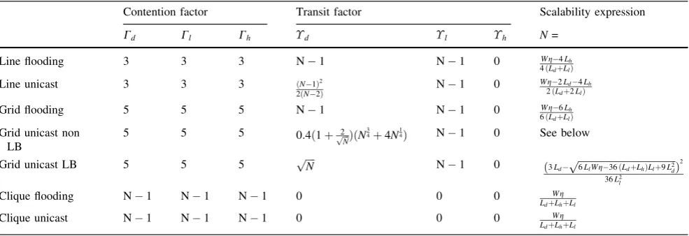
We consider a spatial-reuse TDMA model with node scheduling, also referred to a broadcast scheduling [28] which is an abstraction of real-world TDMA implementa-tions, for example [29]. We use an abstraction rather than a specific TDMA protocol for wider applicability and to avoid results from being tied to peculiarities of specific designs. That is, time is slotted and slots are grouped into repeating frames. Every node is assigned a slot in a frame in which it is allowed to transmit and its neighbors receive. Thus, nodes that are neighbors or share a common neighbor should be assigned different slots. The goal of a TDMA protocol is to perform conflict-free assignment using the least possible number of slots. Our model captures the control overhead—an integral part of any real TDMA implementation—for its operation by means of an addi-tional ‘‘control slot’’ at the beginning of each frame. We assume that the control and data slots are of the same length. The control slot may be further subdivided into mini-slots for control purposes in a protocol-specific way. The signature set for TDMA-based networks is given in Table 2. The first three columns contain the contention factor, and the second three contain the transit factor. The last column is the result of substituting the corresponding
contention and transit factors into Eq.6 and solving for
N. To understand the table, it suffices to explain how we got the contention and transit factors, which we do below for each row.
We note that since Hello packets are only transmitted one hop, the transit factor h is zero for all topologies.
Similarly, a flooded packet is transmitted by every other node in line and grid and hencel isN1, whereas it is
not re-transmitted in clique sol for clique is 0. Thus, we
only consider the first 4 columns of Table2below. Further, for flooding traffic including LSUs, all nodes are equal bottlenecks and therefore the residual capacity of interest is at the bottleneck node for unicast. Without loss of gener-ality we assume an odd number of nodes (for line) and rows and columns (for grid), and therefore the center node as bottleneck.
4.1.1 Line networks
A line network can be node scheduled using 3 slots, for example, using slot numbers 1, 2, and 3 repeating from left to right on the line. Thus, a typical node has to defer for nodes transmitting in slots other than its own and the control slot, and thus the contention factor is 3 for both link-layer unicast and broadcast. Since all traffic uses one of these modes, all of the contention factors are 3.
Consider the transit factor (TF). The TF for flooded data is clearly the same as that of LSUs, and therefore, d¼N1. For the TF of unicast data, we need to
com-pute the expected number of paths that go through b. The probability that a given node routes through b is the probability that the destination lies on the ‘‘other side’’ of
b, that is, pðBÞ ¼ðNN1Þ2=2. Thus, the expected number of paths ispðBÞ ðN1Þas shown.
4.1.2 Grid networks
We consider a grid network of N¼mmnodes. Such a grid network can be scheduled using 5 slots using a straightforward assignment scheme as shown with an example for a 77 grid in Fig.2. This is tight, since there clearly is a 2-hop clique of 5 nodes each of which would need a different color. Thus, our model captures a TDMA protocol that uses 5 slots to color a grid in addition to the control slot.
Consider the contention factor. With node scheduling, the node of interest has to defer for nodes transmitting in 4 slots other than its own, plus the control slot, that is, equivalent of 5 nodes. Thus, the contention factor is 5 in both cases for all traffic.
Consider the transit factor (TF). Clearly, the TF of flooded data is N1 similar to the line. For the TF of 3 An alternate model/assumption would be multiple unicast
unicast data, we need to compute the expected number of paths through the center node b. In the ‘‘Appendix’’, we have derived an approximate formula for the number of
expected paths through the center as 0:4ð1þ 2ffiffiffi
N
p ÞðN34þ
4N14Þ.
Due to the complex radicals in the transit factor, we could derive a closed form forN only using an approxi-mation of the transit factor, and even this is much too long to display in this or any paper. While this does not hamper us from generating numbers for plots using numerical techniques in mathematical software, it does make it cumbersome to work with for insights. Therefore, we have also provided a much simpler closed-form expression using a lower bound for the expected number of paths through the center aspffiffiffiffiN, derived in [20]. This lower bound also happens to correspond to the case when routing does the best possible load balancing of its traffic [20]. Thus, there are two rows—LB (Load Balanced), and Non LB (Non
Load Balanced) in Table2. The Non LB assumes that traffic is forwarded along shortest paths, ties broken ran-domly. Note that this will result in uneven load and when the center node gets saturated, there may still be capacity at the ‘‘edges’’ of the grid. The LB assumes that the routing protocol balances the load, say using the ‘‘row first column next’’ approach in [20]. We shall use both the Non LB and LB models as appropriate in the ensuing sections.
4.1.3 Clique networks
A clique or ‘‘complete’’ network is one in which all nodes are mutually adjacent. Given node scheduling, in both unicast and flooding, every packet is transmitted exactly once. Thus, the symptotics are identical for unicast and flooding. No node is a bottleneck, and so any reference node can be taken. Since every node needs a slot, the CF is clearly N1 for all three traffic types. Also, since no packet is ever relayed, the transit factors are zero for all traffic types.
4.2 802.11 based regular networks
In this section, we develop symptotic expressions for Line, Grid and Clique networks with IEEE 802.11g DCF [30] as the underlying MAC protocol. We assume that link-level unicast transmission is always done via an RTS-CTS-DATA-ACK (RCDA) handshake, and MAC-level broad-cast transmission consists simply of the DATA transmission.
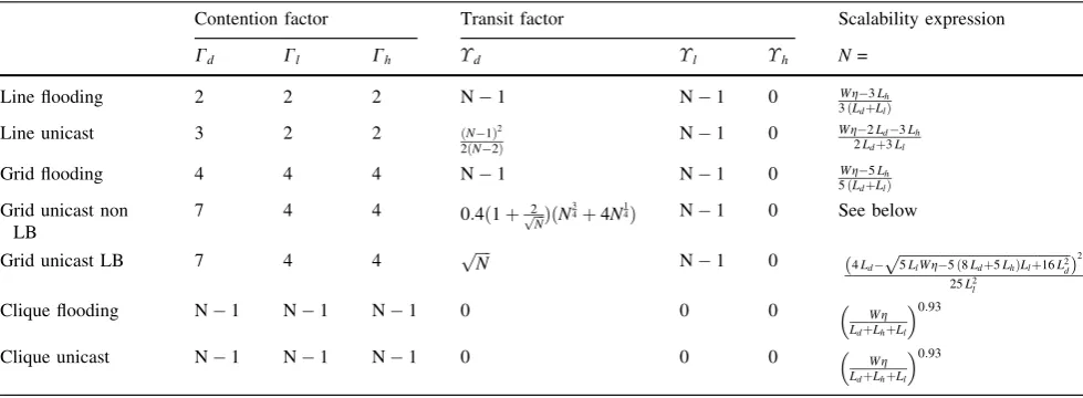
The signature set for 802.11-based networks is given in Table3. We note, however, that the transit behavior as well as the bottleneck node is dependent on the topology and not on the MAC. Hence the transit factors are same as for the corresponding sections in the TDMA section (Table 2). Table 2 Signature set and symptotic scalability expressions for regular networks using TDMA
Contention factor Transit factor Scalability expression
Cd Cl Ch d l h N=
Line flooding 3 3 3 N1 N1 0 Wg4Lh
4ðLdþLlÞ
Line unicast 3 3 3 ðN1Þ2
2ðN2Þ N1 0
Wg2Ld4Lh
2ðLdþ2LlÞ
Grid flooding 5 5 5 N1 N1 0 Wg6Lh
6ðLdþLlÞ
Grid unicast non LB
5 5 5 0:4ð1þ 2ffiffiffi
N
p ÞðN34þ4N14Þ N1 0 See below
Grid unicast LB 5 5 5 pffiffiffiffiN N1 0 3Ld ffiffiffiffiffiffiffiffiffiffiffiffiffiffiffiffiffiffiffiffiffiffiffiffiffiffiffiffiffiffiffiffiffiffiffiffiffiffiffiffi6LlWg36ðLdþLhÞLlþ9L2d p
ð Þ2
36L2 l
Clique flooding N1 N1 N1 0 0 0 Wg
LdþLhþLl
Clique unicast N1 N1 N1 0 0 0 Wg
LdþLhþLl
1 2 3 4 5 1 2
2 3 4
4 5 1
1 2 3
3 4 5
1 2 3 4 4 5 1 2
5 1 2
3 4 5 1 3 4 5
4 1 3 4 5 1
5 1 2 3
2 3 4 5
Therefore, we will only discuss contention factors below, and refer the reader back to Sect.4.1for the explanation of the transit factor part of the signatures.
4.2.1 Line networks
For MAC-layer unicast transmissions, without loss of generality, suppose bottleneck center b wants to send to nodeX. Clearly, due to RTS-CTS based deference behav-ior,b has to defer whenever its neighbors or neighbors of
Xare transmitting, and hence the contention factor is 3. For flooded data, as well as LSAs and Hellos, since MAC-layer broadcast is employed, RTS-CTS are not sent and so node
bneed only desist due to carrier sense which is when either of its neighbors are transmitting.4 Hence CF is 2. It may appear strange that the broadcast contention factor is less than the unicast contention factor, but this merely models the way most real systems (e.g. [31]) work notwithstanding the penalty due to lack of reliability. We note that the actual throughput may be less due to lack of re-transmissions.
4.2.2 Grid networks
Consider the contention factor for bottleneck center node
b. For link-level unicast transmissions, without loss of generality, supposebwants to send to nodeX. Since RTS-CTS is used, all nodes that receive the RTS or the RTS-CTS defer, and by reciprocity, the reference node has a con-tention factor of 7. For link-level broadcast transmissions
(flooding data, LSUs and Hellos), there is no RTS-CTS, and the only deference is via carrier sense, and hence the contention factor is all neighbors, that is, 4.
4.2.3 Clique networks
The signature for clique networks under 802.11 is identical to that for TDMA sinceN1 nodes cause deference by a given node.
However, there are two key factors that come into play with 802.11 that result in different symptotics. First, the overhead causes lower efficiency as discussed earlier. Second, as mentioned earlier, the backoff dynamics cause decreasing efficiency with increasing numbers of nodes. That is, as the probability of collisions and finding the channel busy increase with increasing number of nodes, the efficiency of 802.11 is lower and hence a clique network with 802.11 will scale to less nodes than with TDMA. While this is negligible for fixed degree regular networks such as line and grid, it cannot be ignored for clique as the degree isO(N). This is more thoroughly analyzed in [32], where the efficiency is shown to decrease asN1:08. Using
this, and the signature for 802.11 based clique is as given in the last two rows.
5 Validation
In this section we present results of ns-2 simulations of some of the scenarios analyzed in Sect.4. We instantiate the corresponding symptotic expressions given there and compare them with simulation results for the same set of parameter values (refer Table4). For the link-state routing, we use header parameters from OLSR as a reasonable representative.
4 This is assuming the carrier sense range is same as transmission range. In reality, the carrier sense range depends on the radio. The assumptions is not critical in the context of the framework, that is, should the carrier sense range be two hops, one would merely replace the signature component to 4.
Table 3 Signature set and symptotic scalability expression for regular networks using 802.11
Contention factor Transit factor Scalability expression
Cd Cl Ch d l h N=
Line flooding 2 2 2 N1 N1 0 Wg3Lh
3ðLdþLlÞ
Line unicast 3 2 2 ðN1Þ2
2ðN2Þ N1 0
Wg2Ld3Lh
2Ldþ3Ll
Grid flooding 4 4 4 N1 N1 0 Wg5Lh
5ðLdþLlÞ
Grid unicast non LB
7 4 4 0:4ð1þ 2ffiffiffi
N
p ÞðN34þ4N14Þ N1 0 See below
Grid unicast LB 7 4 4 pffiffiffiffiN N1 0 4Ld ffiffiffiffiffiffiffiffiffiffiffiffiffiffiffiffiffiffiffiffiffiffiffiffiffiffiffiffiffiffiffiffiffiffiffiffiffiffiffiffiffiffiffiffi5LlWg5 8ð Ldþ5LhÞLlþ16L2d p
ð Þ2
25L2 l
Clique flooding N1 N1 N1 0 0 0 Wg
LdþLhþLl
0:93
Clique unicast N1 N1 N1 0 0 0 Wg
LdþLhþLl
For the analytical results, the expressions in the last column of Tables2and3are used. The loadsLd,LlandLh
are calculated based on the sourced packets per second (pps) for each of data (kd), LSU frequency (kl) and Hello
frequency (kh) respectively, the payload size (we use 1000
bytes), and the network and MAC layer headers. For 802.11, the RTS, CTS, and ACK penalty is added when computingLd. The header lengths and variables we use for
the rest of this section are summarized in Table4. The radio rate (W) and the offered flow rate (kd) are variable.
The efficiency (g) is set to 1.0 to model idealized TDMA. In 802.11, the physical layer and MAC layer headers contribute to overhead that results in efficiency g\1. 802.11g uses OFDM and provides raw radio rates from 6 to 54 Mbps. The physical layer preamble is sent at the lowest rate and the contention window slots are fixed length. Thus, the efficiency reduces as the radio rate increases. Based on the derivation given in [15], the datarate (W) to efficiency (g) mappings we use are: (6 Mbps! 0.80), (12 Mbps! 0.70), (24 Mbps!0.58), (54 Mbps!0.40). For rates in between these numbers, the efficiency is linearly interpolated.
We now turn to the simulation set up. The TDMA protocol that we use is an extension of the TDMA model available in the ns-2 distribution. Specifically, we have extended it to a spatial reuse TDMA, that is, one that allows multiple nodes to transmit in the same slot. We then implemented a 3-slot assignment for line networks and a 5-slot assignment for mesh networks as described in Sect.4.1. The TDMA in ns-2 already models a control slot, which we have retained.
For 802.11, we have used the ns-2 model from an overhaul that significantly improves on the original model [33]. The key features include cumulative SINR computation, preamble and PLCP header processing and capture, and frame body capture. The MAC accurately models the basic IEEE 802.11 CSMA/CA mechanism, as required for credible simulation studies. The model implements models of four modulation schemes—BPSK, QPSK, 16-QAM, 64-QAM—with 1/2 coding rate for the first three and 3/4 for 64-QAM to provide four data rates: 6, 12, 24, and 54 Mbps.
The physical layer propagation model is the two-ray groundmodel that is part of the WirelessPHYExt protocol for both TDMA and 802.11. The physical layer settings gives a transmission range of 450 m. To create a line topology, we place nodes separated by a distance of slightly less than 450 m such that only adjacent nodes are within range. Similarly, for a mesh, only nodes adjacent in 4 directions are within range. A clique is formed by ensuring that all nodes are within 450 m of each other. The simulation duration is 30 s, sufficient for static networks.
Each node generates traffic using a Constant Bit Rate (CBR) model. For unicast, a node selects a destination uniformly at random for each packet. For flooding, the packet is sent to all nodes, by broadcasting at the link layer at each node.
We have studied the symptotic scalability Nmax as a
function of pps kd for each of the 12 network scenarios
described in Sect. 4. Per definition 1, at N[Nmax the
residual capacity of at least one node is less than zero. At this point, the input rate on the node’s transmit queue is more than the output, and the queue becomes unstable (that is, starts growing continuously). The ns-2 simulation sys-tem has a finite queue length—therefore, queue instability is detected as packets being dropped due to queue being full. In our simulations, the queue length is 50 packets, and we deem the network saturated if there are non-trivial queue drops, in particular, if there are 50 or more packets dropped.
LetNi denote the network size of a particular run, with
Niþ1[Nifor alli. We run simulations with increasing size
Nitill we encounter two consecutiveNiandNiþ1 such that
there are no queue drops inNiand there are non-trivial ([
50) queue drops in Niþ1. We then measure the symptotic
scalability as the average ofNi andNiþ1. For example, if
there are no queue drops for N=40, and non-trivial drops for N =50, the symptotic scalability is N=45. For the line and clique networks, the increment was 10 nodes and for a mesh, the side was incremented by 1 (i.e., the sizes were 16, 25, 36, 49 and so on).
We have considered alternate measures such as a sudden drop in throughput or increase in delay. The former is fairly unreliable especially for 802.11 networks where collisons cause loss. The latter correlates well with the queue drop measurement, but harder to objectively measure, and hence we have used queue drops as an indication of saturation.
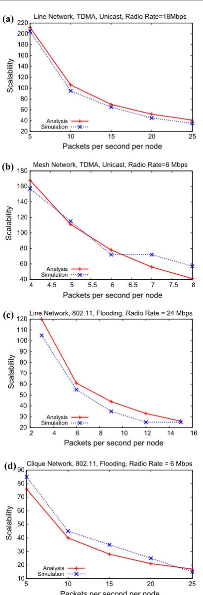
Figure3a–d compare the symptotic scalability predicted by our model with simulation results. Since the simulations take a long time to run for larger sizes, we picked the radio rate and packets per second such that they-axis maximum is not prohibitively large. Further, due to space constraints, we have only shown a subset of the plots, picking a subset such that each topology, MAC and traffic type is repre-sented at least once.
Table 4 Protocol header sizes from [17,34]
Link state routing 802.11
LSU : 52 bytes RTS : 20 bytes Hello : 48 bytes CTS : 14 bytes Net Hdr: 20 bytes ACK : 28 bytes LSU freq(kl) = 0.2 pps MAC Hdr: 28 bytes
Our results show that despite its simplicity and abstraction of details, the scalability predicted by our model matches that predicted by simulations fairly well, and adequately for practical purposes of estimating the rough order of magnitude as motivated in Sect. 1.
The slight discrepancy between the analysis and simula-tion is due to several factors. First, the analysis is approxi-mate by design, and in particular due to simplifications made in the course of the derivations (e.g. assumingN1N), the accuracy is lower for smallerN. On the other hand, we cannot compare using high N because simulations cannot scale to large sizes. Second, for unicast mesh results, we have assumed that routing picks randomly from amongst shortest paths, which may not be the case. Third, for CSMA results, the random processes are only captured in the aggregate. Finally, due to simulation running time constraints, the node step size granularity is high. In particular, in Fig.3(b) the derivation for mesh unicast in ‘‘Appendix’’ is more approx-imate for smallNand therefore we see higher discrepancy at lowerN. In general, due to the approximations introduced for tractability for mesh and due to CSMA being much harder to model than TDMA, the results are best for Line/TDMA.
The simulation results attest to the fact that the approach taken and approximations and assumptions made do not excessively compromise accuracy. The differences seen are within reason, and the slopes parallel for the most part. Our simulation study gives us confidence that our model, despite its simplicity, is adequate for rough order of mag-nitude scalability predictions. In the next two sections, with a validated model in hand, we turn our attention to more complicated and realistic scenarios, and to impact analysis.
6 Other scenarios: randomness and mobility
Thus far we have limited ourselves to topologies that are regular and static. In this section, we relax in a limited way both these constraints. In the next subsection we consider a random topology constrained by real-world connectivity considerations that we term a randomized grid, and in Sect.6.2, we consider a mobile scenario based on a real-world mobility model called repeated traversal mobility. Due to lack of space, we only present expressions with a subset of the MAC and traffic options considered earlier.
6.1 Grid-based random networks
Real-world networks are seldom purely random, that is, with the nodes distributed uniformly randomly in space. Instead, we consider a class of random networks that we call ‘‘Grid Based Random Networks’’ which are formed as follows. First, we partition the network intoMequal-sized 20
40 60 80 100 120 140 160 180 200 220
5 10 15 20 25
Scalability
Packets per second per node
Line Network, TDMA, Unicast, Radio Rate=18Mbps
Analysis Simulation
40 60 80 100 120 140 160 180
4 4.5 5 5.5 6 6.5 7 7.5 8
Scalability
Packets per second per node
Mesh Network, TDMA, Unicast, Radio Rate=6 Mbps
Analysis Simulation
20 30 40 50 60 70 80 90 100 110 120
2 4 6 8 10 12 14 16
Scalability
Packets per second per node
Line Network, 802.11, Flooding, Radio Rate = 24 Mbps
Analysis Simulation
10 20 30 40 50 60 70 80 90
5 10 15 20 25
Scalability
Packets per second per node
Clique Network, 802.11, Flooding, Radio Rate = 6 Mbps
Analysis Simulation
(a)
(b)
(c)
(d)
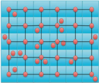
disjoint ‘‘cells’’ and assume that there is at least one node per cell. We assume that nodes in adjacent cells are within communication range of each other. These two assump-tions ensure that a network in this class is always a con-nected network, which is an important criterion for real-world networks. The remaining nodes are located uni-formly at random over the cells. This is illustrated in Fig.4 where it is assumed that nodes in a cell can communicate with nodes in same cell and adjacent cells to the Left, Right, Top, and Bottom. Note that the grid-based random network is an expandable network as defined in Sect.3.1 and hence its symptotic scalability can be analyzed. A grid-based random network could model a community mesh network or a organized deployment of military squads, with a ‘‘cell’’ above modeling a community or a squad, respectively.
We assume there can be at most one concurrent trans-mission per cell and its adjacent cells. Define the node densityqas the ratio of the total number of nodesNto the number of cells M (N¼Mq). Note that q1 since we assume at least one node per cell. The average node density in this network can be controlled by varying this parameter q. Using the signature based analysis for the regular degree-4 grid based on M cells, we can now derive the symptotic scalability expressions this network. Given aq and a traffic demand, we define scalability of this random grid network as the maximum network size N that can support this demand for densityq.
Suppose this network operates according to a spatial-reuse TDMA schedule per the assignment shown in Fig.2. Note that instead of ‘‘node scheduling’’, we have ‘‘cell scheduling’’. Assuming nodes within a cell divide the effective transmission rate equally, the contention factor (CF) and transmit factor (TF) under flooding and unicast for this network can be derived as follows. On average, a node has to contend with 5q1 nodes in its own and neighboring cells. This plus the control slot yields a CF of
Cd ¼Cl¼Ch¼5q for both unicast and broadcast. Next,
consider the transit factor (TF). Similar to regular grid, the TF of Hellos is zero. Assuming that each node in a cell is equally likely to route a flooded packet generated by a node in another cell, we have d¼M1 for flooding while
l¼M1 for both flooding and unicast traffic (where
M¼N=q). Finally, the TF for unicast data can be com-puted using the same procedure as regular grid but now
based on cells, and is given by d¼0:4ð1þp2ffiffiffiMÞðM
3 4þ
4M14Þ for non-load-balanced unicast and byd¼ ffiffiffiffiffiM
p for load balanced unicast.
Using these signatures in the master template, we get the following expression for scalability for flooding traffic.
N¼ Wgq5Lhq
2L
hq
5ðLdþLlÞqþLdþLl
ð7Þ
For load-balanced unicast we get:
N¼2LlWgq
ffiffiffiffiffiffiffiffiffiffiffiffiffiffiffi
5qþ1 p
XLdqY
2 5L2
lqþL2l
ð8Þ
where
X¼
ffiffiffiffiffiffiffiffiffiffiffiffiffiffiffiffiffiffiffiffiffiffiffiffiffiffiffiffiffiffiffiffiffiffiffiffiffiffiffiffiffiffiffiffiffiffiffiffiffiffiffiffiffiffiffiffiffiffiffiffiffiffiffiffiffiffiffiffiffiffiffiffiffiffiffiffiffiffiffiffiffiffiffiffiffiffiffiffiffiffiffiffiffiffiffiffiffiffiffiffiffiffi
4LlWg4ðLdþLhÞLl5 4ðLdþLhÞLlL2d
qþL2
d
q
ð9Þ
Y¼5 2ðLdþLhÞLlL2d
q2 2 L
dþLh
ð ÞLlL2d
q
ð10Þ
As with regular grid, the expression for non-load balanced are much too unwieldy to present. In what follows, we use the load balanced expressions for all numerical computations.
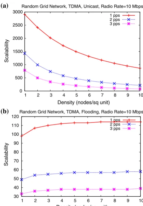
Figure 5 plots the scalability as derived above versus node densityqfor different values of the input traffic load for unicast and flooding respectively. It can be seen that while the scalability decreases withqfor unicast, it initially increases and then appears to converge to a fixed value in case of flooding. These can be explained intuitively as follows. The scalability with increasing q (decreasing
M¼N=q) is governed by a tension between gains from reduced traffic and loss from increased contention. In the case of unicast, the gains from reduced traffic is OðpffiffiffiffiffiMÞ whereas loss from increased contention is O(M), resulting in a decrease with increasingq.5For flooding on the other hand, the corresponding numbers are the same, namely,
O(M) and therefore the scalability is independent ofq. The slight increase for smaller values of qis because we have assumed one control slot for TDMA irrespective ofq and this overhead decreases with increasingqmore discernibly for smaller values ofq.
Fig. 4 Illustration of the degree 4 random grid network model 5 More precisely,NkO
ffiffiffiN
q
q
N=q)NO 1
k2q
An interesting question which we are now in a position to answer is: which is better, a regular grid or a random grid? Due to the way we construct the random grid withN
depending onq, this is better answered by comparing the per-node capacity (throughputLd) of each for varying N.
Using symptotic analysis, we can derive the following expression for maximum per node load for unicast traffic for the random grid model:
Ld ¼
Wgð5LlqþLlÞM5LhqLh
5qþ1
ð ÞpffiffiffiffiffiMþ5qþ1 ð11Þ
Similarly, we can derive the following expression for maximum per node load for flooding for the random grid model:
Ld ¼
Wgð5LlqþLlÞM5LhqLh
5qþ1
ð ÞM ð12Þ
Figure6 shows the comparison between random and reg-ular grid. For the random grid model, we fix the number of cells M¼100 and then calculate the maximum feasible input rate per node for increasing values of q using the
expression above. For regular degree-4 grid, we calculate the same quantity assuming a network of sizeMq, by using Eq. 6 but solving for Ld instead of for N as we did in
Sect.4. Thus, we compare same-sized network in both cases, with size increasing on the X axis. It can be seen from Fig.6(a) that regular degree-4 grid outperforms ran-dom grid network for the same network size under unicast traffic. Intuitively, this also follows from the results of Gupta-Kumar [2] that suggest that for uniform unicast traffic, maximizing the number of concurrent transmissions by keeping transmission range as small as possible (while ensuring network connectivity) is optimal.
However, unlike unicast, we find that for flooding ran-dom grid slightly outperforms regular grid [Fig.6(b)]. Note that a pure asymptotic analysis would conclude that there is no performance gap in this case.
6.2 Mobile networks
In this section, we use the symptotics framework to analyze a real-world mobility scenario often used in tactical net-works (vice a synthetic one such as ‘‘random waypoint’’
0 1 2 3 4 5 6 7 8 9
100 200 300 400 500 600 700 800 900 1000
Max PPS per node
Network size (nodes/sq unit)
Random vs Regular, TDMA, Unicast, Radio Rate=10 Mbps
Regular Grid Random Grid
0 0.1 0.2 0.3 0.4 0.5 0.6 0.7 0.8 0.9 1
100 200 300 400 500 600 700 800 900 1000
Max PPS per node
Network size (nodes/sq unit)
Random vs Regular, TDMA, Flooding, Radio Rate=10 Mbps
Regular Grid Random Grid
(a)
(b)
Fig. 6 Throughput versus size for random grid and regular grid for unicast (a) and flooding (b). Random grid does worse than regular grid with unicast, but interestingly does better with flooding 0
500 1000 1500 2000 2500 3000
1 2 3 4 5 6 7 8 9 10
Scalability
Density (nodes/sq unit)
Random Grid Network, TDMA, Unicast, Radio Rate=10 Mbps
1 pps 2 pps 3 pps
30 40 50 60 70 80 90 100 110 120
1 2 3 4 5 6 7 8 9 10
Scalability
Density (nodes/sq unit)
Random Grid Network, TDMA, Flooding, Radio Rate=10 Mbps
1 pps 2 pps 3 pps
(a)
(b)
which seldom exists in real-life). Specifically, we study the
repeated traversal[35] mobility, as described in the next section.
The repeated traversal mobility model consists of two groups, called theleading group, and thefollowing group. Initially, the groups are co-located. The leading group moves first and rests, after which the following group moves and joins the leading group. The process then repeats itself. Repeated traversal is prevalent in military troops through hostile terrain, where the leading squad of soldiers clears the terrain of threats before the following squad follows. The model is also applicable to civilian scenarios, notably disaster relief. An example of repeated traversal is depicted in Fig.7.
Note that a network with repeated traversal mobility is an expandable network as defined in Sect.3.1and hence its symptotic scalability can be analyzed. We study a specific case of the repeated traversal depicted in Fig.7 in which each group is arranged in a line, as might be the case when the groups are disaster relief convoys. We assume that the two groups are identical in terms of group size and node density. Specifically, distances between consecutive nodes are identical throughout each group. Moreover, we also assume that inter-group distances are significantly larger than intra-group distances, and the communication range of each node is such that it can reach all nodes in its group in one hop. Note that while the connectivity within each group is a ‘‘clique network’’, the fact that the nodes are in a line means that inter-group connectivity changes happen in a step-by-step manner than all at once. This is depicted in Fig.8.
Figure 8 also demonstrates the specific stages of dif-ferent connectivity for the case when the leading group moves away from the following group, resulting in link breakages. For lack of space only T=0 to T¼M1 are shown. The pattern from then to T¼2M1, and the second part when the following group recovers the distance and links are created are similar in nature.
When both groups are in full communication range at the beginning of the movement, the overall network con-nectivity is a giant clique. As the leading group moves, after some time, some pairs of nodes from separate groups start to lose direct contact, leading to a different topology. During these stages, multi-hop relaying is required to communicate between nodes in different groups. Ulti-mately, when the groups are completely isolated, the net-work consists of two disjoint cliques.
The overall effect of mobility on symptotic scalability is two-fold: (1) Different stages of connectivity throughout movement results in different signaturesðCjðtÞ; jðtÞÞfor
each stage; and (2) Link breakages and creations necessi-tate exchange of Link Snecessi-tate Updates (LSU), increasing
control overhead. The amount of LSU packets required depend on the number of link breakages or creations, hence potentially vary with the specific stage. Moreover, ðClðtÞ; lðtÞÞalso potentially depend on the stage number,
since relaying options are changed.
The analysis for repeated traversal mobility depends upon whether the traffic is unicast or flooding. In this paper, we focus primarily on the flooding case. An analysis for unicast has been developed by us in [36] and summa-rized at the end of the discussion on flooding.
We present the signatures of the network for the kth stage number in Table 5for flooding traffic, where stages increment with change of topology. The signatures of the stages where the following group recovers the distance and connects again with the leading group is identical, only as a reverse sequence of the above.
For flooding, contention factors depend on number of neighbors as in static case and all traffic types have equal contention factors. However, transit factors vary for dif-ferent traffic types. For data packets, every node creates packets. On the other hand, since the link-state routing is Fig. 7 Stages and connectivity of Repeated Traversal of convoy groups. Gf, Gl represent the following and leading groups
respec-tively.Gl starts moving at time T=0,Gf at time T=tp,Gl stops
moving at time T =t1
event-driven per our assumption, for LSU packets, only nodes which experience link breakages or formations send out control packets, hence LSU traffic generated each stage changes with movement stage, resulting in lower transit factors. Specifically, LSU traffic initially increases with stage number due to increasing number of link breakages and is maximized at stageM1. Afterwards, the number of nodes from different groups that are in contact starts to reduce gradually, also reducing the number of link break-ages and LSU traffic accordingly.
We now derive the symptotic scalability expression for repeated traversal. From Eq.6and Table5, and noting that signatures are now a function of both the stagekand the group sizeM, we have
gW ¼ ð1þCdðM;kÞÞLdð1þdðM;kÞÞ
þ ð1þClðM;kÞÞLlð1þlðM;kÞÞ
þ ð1þChðM;kÞÞLdð1þhðM;kÞ
ð13Þ
for8ksuch that 0k2M1, resulting in 2Mequations for a given group sizeM.
We first fixM and investigate which stagekmaximizes the RHS of (13), that is, determine the bottleneck node and stage. It is easily seen that the bottleneck stage is one of the intermediate stages between disconnected and fully con-nected network. Note that per definition1 and related dis-cussion thereof, the lack of traffic across the groups does not mean that the symptotic scalability is zero. Of these stages, it is clear that the contention factor for nodes that are closer to the other group is larger. Additionally, these nodes also have a higher transit factor, since they provide relaying for the farther nodes. As a result, at each intermediate stage, the two nodes from each group that are closest to the other group are the bottlenecks. In particular, we observe that the largest amount of loading occurs at stageM1, which corresponds to the instance when only one member of each group still has contact with the other group as well.
Plugging in the signatures at k¼M1, we have the following equation to characterize the scalable network size:
gW ¼2MLd2Mþ2MLl2Mþ2MLh ð14Þ
Since network sizeN¼2M, we have
gW ¼N2LdþN2LlþNLh¼N2ðLdþLlÞ þNLh ð15Þ
Solving the quadratic equation for N and taking the only non-negative solutions, we have
N¼
ffiffiffiffiffiffiffiffiffiffiffiffiffiffiffiffiffiffiffiffiffiffiffiffiffiffiffiffiffiffiffiffiffiffiffiffiffiffi L2
hþ4gWðLdþLlÞ
p
Lh
2ðLdþLlÞ
ffiffiffiffiffiffiffiffiffiffiffiffiffiffiffi
gW LdþLl
r
: ð16Þ
for LdþLl Lh.
How does this compare with static scenarios? Recall that the scalability of the closest static analogues, namely the line and the clique network was approximatelyN gW
ðLdþLlÞ (refer Sect.4.1) which implies a linear increase in scalable size with radio rate. In contrast, we now have, from Eq. (16) a square root dependence for repeated traversal. In other words, to double the supported number of nodes, roughly the radio rate must be increased four times vice two times for static. On the other hand, Eq. (16) also reveals that the dependence between traffic load and
scal-able group size is roughly given byNaðLdþLlÞ0:5, hence
doubling the load only reduces scalable size by about 30 % vice halving it for static.
We use the parameters from Table4 in Sect. 5, with radio rate W set to 10 Mbps for all plots where it is not varied and the flow rate per node set to 1 pps for all plots where it is not varied.
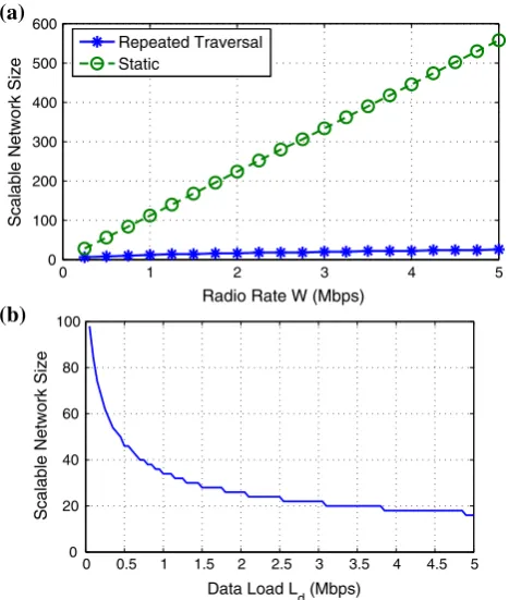
Figure9(a) plots the scalable network size as a function of radio rateWfor both static and repeated traversal. First, we observe that repeated traversal reduces scalability by more than an order of magnitude. Specifically, for W = 2 Mbps, the scalability falls from 224 nodes for static to a mere 16 nodes for repeated traversal. Since contention factor for the static case is equal toN1, it is apparent that this decrease is due to the increase in transit factorsd
andl, in particular, at the bottleneck nodes at the edge in
stageM1.
Finally, for fixed radio rateW¼10 Mbps we vary data traffic loadkd in Fig. 9(b). Also, as expected, the scalable
group size does not reduce to half when load is doubled, but is rather larger, around the 70 % as provisioned.
In sum, we have provided expressions for the scalability of repeated traversal for flooding traffic. We show that contrary to asymptotic results [3], mobility in certain sce-narios reduces capacity and hence scalability in the Table 5 Stages of repeated
traversal and their signatures Mvmt Stage,k CdðkÞ ClðkÞ ChðkÞ dðkÞ lðkÞ
k¼0 2M1 2M1 2M1 0 0
1k M1 2M1 2M1 2M1 2k 2k
Mk 2M1 2M1 3M1k 3M1k 2M1 2ð2MkÞ
k¼2M M1 M1 M1 0 0
symptotic regime. The main reason is the change in topology, and increased traffic in some specific nodes, which are the bottleneck nodes. Further, N varies as the square root of radio rate and the inverse square root of the load, which is asymptotically distinct from static where the relationship is linear.
We conclude by briefly summarizing the results on the unicast case. As mentioned earlier, we have detailed our results in [36]. Different from the flooding case, the unicast scenario also addresses issues as dynamic routing and route re-discovery due to mobility. In particular, due to the changing topologies and connectivity, the best (if more than one exists) route between a given source and desti-nation node also potentially changes and has to be updated (discovered) after each movement stage. As one would expect, this increases both the complexity in operational and the derivation of the transit factors of bottleneck nodes. In order to provide insight, here we provide a brief summary of such results. In particular, in [36] we consider two different routing protocols, one choosing any of the existing routes with minimum hop count with equal prob-ability, and one which aims to be energy efficient by equalizing hop lengths. Depending on the movement stage, the minimum number of hops that you can reach a given source-destination pair can be either one, two, or three. In
particular the cases where at least two or three hops exist are more interesting, and depending on the associated routes, it is possible to characterize the transit factor of the bottleneck nodes for data traffic and LSU traffic. The TF expressions turn out to be notably more involved [36], and are also a function of the mobility stage, and group size, quite often involving Harmonic numbers.
Despite the fact that the bottleneck stage can occasion-ally differ in certain special cases where data traffic is light compared with the flooding case, we also observe that in general there exists a square-root dependence between scalability and bandwitdh for unicast traffic as well [36]. In sum, those results along with the flooding results provided above comprise a full treatment of user mobility with both unicast and flooding traffic, including considerations of route re-discovery, and demonstrate that the framework can accommodate real-world user mobility.
7 Impact analysis
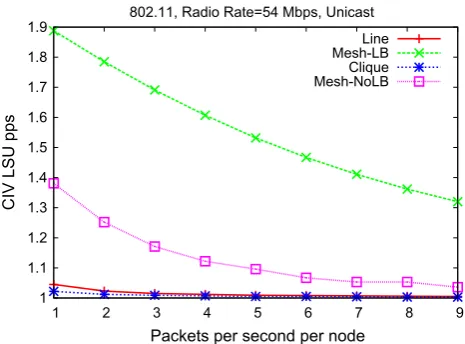
In this section, we introduce the concept ofchange impact valuefor quantifying the impact of a particular parameter such as routing overhead, radio rate, or offered load on scalability, and illustrate how it can be used along with the symptotic models derived in the previous sections to drive design choices to meet a scaling requirement. We then study how their impact changes with nominal values of other network parameters.
7.1 Change impact value
In Sect.4, we derived several expressions of the formN¼
fðXÞwhereX¼ ðx1;x2;. . .;xnÞis the parameter vector on
whichNdepends. For example, in the symptotic scalability of a line network using TDMA and flooding, namely,
N¼Wg4Lh
4ðLdþLlÞ,X¼W;g;Lh;Ld;Ll. These parameters define the scalability region for the network in question. The value of N for a specific network scenario obviously depends upon the values of the parameters.
A real-world system typically has a set of default or
nominal parameters, for instance, as part of its initial configuration. LetVdenote thenominal instantiationof the parameter vector X, with ðx1¼v1;x2¼v2;. . .;xn¼vnÞ,
where vi is the nominal or default value of parameter xi.
Further, letVxj¼krepresent that parameterxjisover-ridden with valuekinV, while all other parameters are as in the nominal instantiation.
Definition 3 The Change Impact Value of parameter xj
for a ‘‘change factor’’a isCIVðxj;aÞ= fðVxj¼avjÞ
fðVÞ .
0 1 2 3 4 5
0 100 200 300 400 500 600
Radio Rate W (Mbps)
Scalable Network Size
Repeated Traversal Static
0 0.5 1 1.5 2 2.5 3 3.5 4 4.5 5 0
20 40 60 80 100
Data Load L d (Mbps)
Scalable Network Size
(a)
(b)
![Table 4 Protocol header sizes from [17, 34]](https://thumb-us.123doks.com/thumbv2/123dok_us/586486.2057875/10.595.52.290.72.158/table-protocol-header-sizes-from.webp)