27Giancoli Ch 27 Atomic

C

H

A

P

T

E

R

Early Quantum Theory

and Models of the Atom

It has been found experimentally that (a) light behaves as a wave.

(b) light behaves as a particle. (c) electrons behave as particles. (d) electrons behave as waves. (e) all of the above are true. (f) only (a) and (b) are true. (g) only (a) and (c) are true. (h) none of the above are true.

T

771

CONTENTS

27–1 Discovery and Properties of the Electron

27–2 Blackbody Radiation; Planck’s Quantum Hypothesis

27–3 Photon Theory of Light and the Photoelectric Effect

27–4 Energy, Mass, and Momentum of a Photon

*27–5 Compton Effect

27–6 Photon Interactions; Pair Production

27–7 Wave–Particle Duality; the Principle of Complementarity

27–8 Wave Nature of Matter

27–9 Electron Microscopes

27–10 Early Models of the Atom

27–11 Atomic Spectra: Key to the Structure of the Atom

27–12 The Bohr Model

27–13 de Broglie’s Hypothesis Applied to Atoms

27

just as light does. Because the wavelength of electrons can be much smaller than that of visible light, much greater resolution and magnification can be obtained. A scanning electron microscope (SEM) can produce images with a three-dimensional quality.

27–1

Discovery and Properties of

the Electron

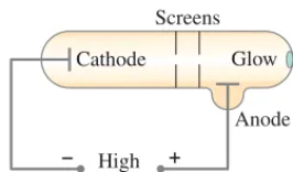
Toward the end of the nineteenth century, studies were being done on the discharge of electricity through rarefied gases. One apparatus, diagrammed in Fig. 27–1, was a glass tube fitted with electrodes and evacuated so only a small amount of gas remained inside. When a very high voltage was applied to the electrodes, a dark space seemed to extend outward from the cathode (negative electrode) toward the opposite end of the tube; and that far end of the tube would glow. If one or more screens containing a small hole were inserted as shown, the glow was restricted to a tiny spot on the end of the tube. It seemed as though something being emitted by the cathode traveled across to the opposite end of the tube. These “somethings” were named cathode rays.

There was much discussion at the time about what these rays might be. Some scientists thought they might resemble light. But the observation that the bright spot at the end of the tube could be deflected to one side by an electric or magnetic field suggested that cathode rays were charged particles; and the direction of the deflection was consistent with a negative charge. Furthermore, if the tube con-tained certain types of rarefied gas, the path of the cathode rays was made visible by a slight glow.

Estimates of the charge e of the cathode-ray particles, as well as of their charge-to-mass ratio had been made by 1897. But in that year, J. J. Thomson (1856–1940) was able to measure directly, using the apparatus shown in Fig. 27–2. Cathode rays are accelerated by a high voltage and then pass between a pair of parallel plates built into the tube. Another voltage applied to the parallel plates produces an electric field and a pair of coils produces a magnetic field BB. If E = B = 0, the cathode rays follow path b in Fig. 27–2.

EB, e兾m e兾m,

FIGURE 27–1 Discharge tube. In some models, one of the screens is the anode (positive plate).

High voltage Cathode

Screens

Glow

Anode

– +

FIGURE 27–2 Cathode rays deflected by electric and magnetic fields. (See also Section 17–11 on the CRT.)

I

High

voltage Electric field

plates Coils to produce

magnetic field

Anode I

a

c b

–

– – –

+ + +

+ +

When only the electric field is present, say with the upper plate positive, the cathode rays are deflected upward as in path a in Fig. 27–2. If only a magnetic field exists, say inward, the rays are deflected downward along path c. These observations are just what is expected for a negatively charged particle. The force on the rays due to the magnetic field is where eis the charge and vis the velocity of the cathode rays (Eq. 20–4). In the absence of an electric field, the rays are bent into a curved path, and applying Newton’s second law

with acceleration gives

and thus

The radius of curvature rcan be measured and so can B. The velocity vcan be found by applying an electric field in addition to the magnetic field. The electric

e

m = Brv .

evB = mv_r2, a = centripetal

F = ma

fieldEis adjusted so that the cathode rays are undeflected and follow path b in Fig. 27–2. In this situation the upward force due to the electric field, is balanced by the downward force due to the magnetic field, We equate the two forces, and find

Combining this with the above equation we have

(27;1)

The quantities on the right side can all be measured, and although eandmcould not be determined separately, the ratio could be determined. The accepted

value today is Cathode rays soon came to be called

electrons.

Discovery in Science

The “discovery” of the electron, like many others in science, is not quite so obvious as discovering gold or oil. Should the discovery of the electron be credited to the person who first saw a glow in the tube? Or to the person who first called them cathode rays? Perhaps neither one, for they had no conception of the electron as we know it today. In fact, the credit for the discovery is generally given to Thomson, but not because he was the first to see the glow in the tube. Rather it is because he believed that this phenomenon was due to tiny negatively charged particles and made careful measurements on them. Furthermore he argued that these particles were constituents of atoms, and not ions or atoms themselves as many thought, and he developed an electron theory of matter. His view is close to what we accept today, and this is why Thomson is credited with the “discovery.” Note, however, that neither he nor anyone else ever actually saw an electron itself. We discuss this briefly, for it illustrates the fact that discovery in science is not always a clear-cut matter. In fact some philosophers of science think the word “discovery” is often not appropriate, such as in this case.

Electron Charge Measurement

Thomson believed that an electron was not an atom, but rather a constituent, or part, of an atom. Convincing evidence for this came soon with the determin-ation of the charge and the mass of the cathode rays. Thomson’s student J. S. Townsend made the first direct (but rough) measurements of ein 1897. But it was the more refined oil-drop experimentof Robert A. Millikan (1868–1953) that yielded a precise value for the charge on the electron and showed that charge comes in discrete amounts. In this experiment, tiny droplets of mineral oil carrying an electric charge were allowed to fall under gravity between two parallel plates, Fig. 27–3. The electric field Ebetween the plates was adjusted until the drop was suspended in midair. The downward pull of gravity,mg, was then just balanced by the upward force due to the electric field. Thus so the charge

The mass of the droplet was determined by measuring its terminal velocity in the absence of the electric field. Often the droplet was charged negatively, but some-times it was positive, suggesting that the droplet had acquired or lost electrons (by friction, leaving the atomizer). Millikan’s painstaking observations and analysis pre-sented convincing evidence that any charge was an integral multiple of a smallest charge,e, that was ascribed to the electron, and that the value of ewas

This value of e, combined with the measurement of gives the mass of the

electron to be This mass is

less than a thousandth the mass of the smallest atom, and thus confirmed the idea that the electron is only a part of an atom. The accepted value today for the mass of the electron is

The experimental result that any charge is an integral multiple of emeans that electric charge is quantized(exists only in discrete amounts).

me = 9.11 * 10–31kg.

9.1 *10–31_kg.

A1.6 * 10–19_{CB兾A1.76 * 10}11_{C兾kgB =} e兾m

,

1.6 * 10–19_C.

q = mg兾E.

qE = mg

e兾m = 1.76 * 1011_C兾kg.e兾m

e

m = BE2_r.

v = E

B.

eE = evB,

F = evB.

F = eE,

SECTION 27–1

773

– –

Atomizer

Droplets

Telescope

– –

+ +

27–2

Blackbody Radiation;

Planck’s Quantum Hypothesis

Blackbody Radiation

One of the observations that was unexplained at the end of the nineteenth cen-tury was the spectrum of light emitted by hot objects. We saw in Section 14–8 that all objects emit radiation whose total intensity is proportional to the fourth power of the Kelvin (absolute) temperature At normal temperatures we are not aware of this electromagnetic radiation because of its low intensity. At higher temperatures, there is sufficient infrared radiation that we can feel heat if we are close to the object. At still higher temperatures (on the order of 1000 K), objects actually glow, such as a red-hot electric stove burner or the heating element in a toaster. At temperatures above 2000 K, objects glow with a yellow or whitish color, such as white-hot iron and the filament of a lightbulb. The light emitted contains a continuous range of wavelengths or frequencies, and the spectrum is a plot of intensity vs. wavelength or frequency. As the temperature increases, the electromagnetic radiation emitted by objects not only increases in total intensity but has its peak intensity at higher and higher frequencies.

The spectrum of light emitted by a hot dense object is shown in Fig. 27–4 for an idealized blackbody. A blackbody is a body that, when cool, would absorb all the radiation falling on it (and so would appear black under reflection when illuminated by other sources). The radiation such an idealized blackbody would emit when hot and luminous, called blackbody radiation(though not necessarily black in color), approximates that from many real objects. The 6000-K curve in Fig. 27–4, corresponding to the temperature of the surface of the Sun, peaks in the visible part of the spectrum. For lower temperatures, the total intensity drops considerably and the peak occurs at longer wavelengths (or lower frequencies). This is why objects glow with a red color at around 1000 K. It is found experimen-tally that the wavelength at the peak of the spectrum, is related to the Kelvin temperatureT by

(27;2) This is known as Wien’s law.

The Sun’s surface temperature. Estimate the tempera-ture of the surface of our Sun, given that the Sun emits light whose peak intensity occurs in the visible spectrum at around 500 nm.

APPROACH We assume the Sun acts as a blackbody, and use in

Wien’s law (Eq. 27–2).

SOLUTION Wien’s law gives

Star color. Suppose a star has a surface temperature of 32,500 K. What color would this star appear?

APPROACH We assume the star emits radiation as a blackbody, and solve for

in Wien’s law, Eq. 27–2.

SOLUTION From Wien’s law we have

The peak is in the UV range of the spectrum, and will be way to the left in Fig. 27–4. In the visible region, the curve will be descending, so the shortest visible wavelengths will be strongest. Hence the star will appear bluish (or blue-white).

NOTE This example helps us to understand why stars have different colors (reddish for the coolest stars; orangish, yellow, white, bluish for “hotter” stars.)

lP =

2.90 * 10–3_mK

T =

2.90 * 10–3_mK

3.25 * 104_K = 89.2nm.

lP

EXAMPLE 27;2

T = 2.90 * 10_l –3mK

P =

2.90 * 10–3_mK

500 * 10–9_m L 6000K.

lP = 500nm EXAMPLE 27;1

lPT = 2.90 * 10–3mK.

lP,

(L 300K),

AT4_B.

FIGURE 27–4 Measured spectra of wavelengths and frequencies emitted by a blackbody at three different temperatures.

0

Wavelength (nm) Frequency (Hz)

1000 2000 3000

Visible IR UV

Intensity

3000 K 4500 K

6000 K 3.0

1014

1.0

Planck’s Quantum Hypothesis

In the year 1900, Max Planck (1858–1947) proposed a theory that was able to reproduce the graphs of Fig. 27–4. His theory, still accepted today, made a new and radical assumption: that the energy of the oscillations of atoms within molecules cannot have just any value; instead each has energy which is a multiple of a mini-mum value related to the frequency of oscillation by

Here h is a new constant, now called Planck’s constant, whose value was estimated by Planck by fitting his formula for the blackbody radiation curve to experiment. The value accepted today is

Planck’s assumption suggests that the energy of any molecular vibration could be only a whole number multiple of hf:

(27;3) where nis called a quantum number(“quantum” means “discrete amount” as opposed to “continuous”). This idea is often called Planck’s quantum hypothesis, although little attention was brought to this point at the time. In fact, it appears that Planck considered it more as a mathematical device to get the “right answer” rather than as an important discovery. Planck himself continued to seek a classical explanation for the introduction of h. The recognition that this was an important and radical innovation did not come until later, after about 1905 when others, particularly Einstein, entered the field.

The quantum hypothesis, Eq. 27–3, states that the energy of an oscillator can be or 2hf, or 3hf, and so on, but there cannot be vibrations with energies between these values. That is, energy would not be a continuous quan-tity as had been believed for centuries; rather it is quantized—it exists only in discrete amounts. The smallest amount of energy possible (hf) is called the quantum of energy. Recall from Chapter 11 that the energy of an oscillation is proportional to the amplitude squared. Another way of expressing the quantum hypothesis is that not just any amplitude of vibration is possible. The possible values for the amplitude are related to the frequency f .

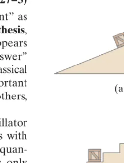
A simple analogy may help. Compare a ramp, on which a box can be placed at any height, to a flight of stairs on which the box can have only certain discrete amounts of potential energy, as shown in Fig. 27–5.

27–3

Photon Theory of Light and

the Photoelectric Effect

In 1905, the same year that he introduced the special theory of relativity, Einstein made a bold extension of the quantum idea by proposing a new theory of light. Planck’s work had suggested that the vibrational energy of molecules in a radiat-ing object is quantized with energy where nis an integer and fis the frequency of molecular vibration. Einstein argued that when light is emitted by a molecular oscillator, the molecule’s vibrational energy of nhfmust decrease by an amounthf(or by 2hf, etc.) to another integer times hf, such as Then to conserve energy, the light ought to be emitted in packets, or quanta, each with an energy

(27;4)

wherefis here the frequency of the emitted light. Again his Planck’s constant. Because all light ultimately comes from a radiating source, this idea suggests that light is transmitted as tiny particles, or photonsas they are now called, as well as via the waves predicted by Maxwell’s electromagnetic theory. The photon theory of light was also a radical departure from classical ideas. Einstein proposed a test of the quantum theory of light: quantitative measurements on the photoelectric effect.

E = hf,

(n - 1)hf.

E = nhf,

E = hf,

E = nhf,

E = hf.

SECTION 27–3 Photon Theory of Light and the Photoelectric Effect

775

FIGURE 27–5 Ramp versus stair analogy. (a) On a ramp, a box can have continuous values of potential energy. (b) But on stairs, the box can have only discrete (quantized) values of energy.

(a)

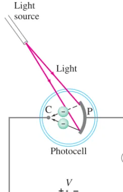
When light shines on a metal surface, electrons are found to be emitted from the surface. This effect is called the photoelectric effect and it occurs in many materials, but is most easily observed with metals. It can be observed using the apparatus shown in Fig. 27–6. A metal plate P and a smaller electrode C are placed inside an evacuated glass tube, called a photocell. The two electrodes are connected to an ammeter and a source of emf, as shown. When the photocell is in the dark, the ammeter reads zero. But when light of sufficiently high frequency illuminates the plate, the ammeter indicates a current flowing in the circuit. We explain completion of the circuit by imagining that electrons, ejected from the plate by the impinging light, flow across the tube from the plate to the “collector” C as indicated in Fig. 27–6.

That electrons should be emitted when light shines on a metal is consistent with the electromagnetic (EM) wave theory of light: the electric field of an EM wave could exert a force on electrons in the metal and eject some of them. Einstein pointed out, however, that the wave theory and the photon theory of light give very different predictions on the details of the photoelectric effect. For example, one thing that can be measured with the apparatus of Fig. 27–6 is the maximum kinetic energy of the emitted electrons. This can be done by using a variable voltage source and reversing the terminals so that electrode C is negative and P is positive. The electrons emitted from P will be repelled by the negative electrode, but if this reverse voltage is small enough, the fastest electrons will still reach C and there will be a current in the circuit. If the reversed voltage is increased, a point is reached where the current reaches zero—no electrons have sufficient kinetic energy to reach C. This is called the stopping potential, or stoppingvoltage, and from its measurement, can be determined using conservation of energy (loss of in potential energy):

Now let us examine the details of the photoelectric effect from the point of view of the wave theory versus Einstein’s particle theory.

First the wave theory, assuming monochromatic light. The two important properties of a light wave are its intensity and its frequency (or wavelength). When these two quantities are varied, the wave theory makes the following predictions:

1. If the light intensity is increased, the number of electrons ejected and their maximum kinetic energy should be increased because the higher intensity means a greater electric field amplitude, and the greater electric field should eject electrons with higher speed.

2. The frequency of the light should not affect the kinetic energy of the ejected electrons. Only the intensity should affect

The photon theory makes completely different predictions. First we note that in a monochromatic beam, all photons have the same energy Increasing the intensity of the light beam means increasing the number of photons in the beam, but does not affect the energy of each photon as long as the frequency is not changed. According to Einstein’s theory, an electron is ejected from the metal by a collision with a single photon. In the process, all the photon energy is trans-ferred to the electron and the photon ceases to exist. Since electrons are held in the metal by attractive forces, some minimum energy is required just to get an electron out through the surface. is called the work function, and is a few electron volts for most metals. If the frequency fof the incoming light is so low that hf is less than then the photons will not have enough energy to eject any electrons at all. If then electrons will be ejected and energy will be conserved in the process. That is, the input energy (of the photon),hf, will equal the outgoing kinetic energy of the electron plus the energy required to get it out of the metal,W:

(27;5a)

The least tightly held electrons will be emitted with the most kinetic energy Ake_maxB,

hf = ke + W.

ke hf 7 W0,

W0,

A1eV = 1.6 * 10–19_JBW0

W0

(= hf).

ke_max.

ke_max = eV0.

kinetic energy = gain

ke_max

V0,

Ake_maxB

Wave

theory

predictions FIGURE 27–6 The photoelectric effect.

+ –

C _P

Photocell Light Light

source

A

V

in which case W in this equation becomes the work function and becomes

[least bound electrons] (27;5b)

Many electrons will require more energy than the bare minimum to get out of the metal, and thus the kinetic energy of such electrons will be less than the maximum.

From these considerations, the photon theory makes the following predictions:

1. An increase in intensity of the light beam means more photons are incident, so more electrons will be ejected; but since the energy of each photon is not changed, the maximum kinetic energy of electrons is not changed by an increase in intensity.

2. If the frequency of the light is increased, the maximum kinetic energy of the electrons increases linearly, according to Eq. 27–5b. That is,

This relationship is plotted in Fig. 27–7.

3. If the frequency fis less than the “cutoff” frequency where no electrons will be ejected, no matter how great the intensity of the light.

These predictions of the photon theory are very different from the predictions of the wave theory. In 1913–1914, careful experiments were carried out by R. A. Millikan. The results were fully in agreement with Einstein’s photon theory.

One other aspect of the photoelectric effect also confirmed the photon theory. If extremely low light intensity is used, the wave theory predicts a time delay before electron emission so that an electron can absorb enough energy to exceed the work function. The photon theory predicts no such delay—it only takes one photon (if its frequency is high enough) to eject an electron—and experiments showed no delay. This too confirmed Einstein’s photon theory.

Photon energy. Calculate the energy of a photon of blue light, in air (or vacuum).

APPROACH The photon has energy (Eq. 27–4) where

(Eq. 22–4).

SOLUTION Since we have

or (See definition of eV in

Section 17–4, )

Photons from a lightbulb. Estimate how many visible light photons a 100-W lightbulb emits per second. Assume the bulb has a typical efficiency of about 3%(that is, 97%of the energy goes to heat).

APPROACH Let’s assume an average wavelength in the middle of the visible

spectrum, The energy of each photon is Only

3%of the 100-W power is emitted as visible light, or The number of photons emitted per second equals the light output of divided by the energy of each photon.

SOLUTION The energy emitted in one second is where Nis

the number of photons emitted per second and Hence

per second, or almost 1019photons emitted per second, an enormous number.

N = _hfE = E_hcl = (3J)A500 * 10

–9

mB

A6.63 * 10–34_{JsBA3.00 * 10}8_m兾sB L 8 * 10 18

f = c兾l.

E = Nhf

(= 3J)

3J兾s 3W = 3J兾s.

E = hf = hc兾l. l L 500nm.

EXAMPLE 27;4 ESTIMATE 1eV = 1.60 * 10–19_J.

A4.4 * 10–19_JB

兾

E = hf = hc_l = A6.63 * 10

–34

JsBA3.00 * 108m兾sB

A4.5 * 10–7_mB = 4.4 * 10

–19_J,

f = c兾l,

f = c兾l

E = hf

l = 450nm

EXAMPLE 27;3

hf0 = W0,

f0,

ke_max = hf - W0.

AW0B

hf = ke_max + W0.

ke_max:

ke W0,

SECTION 27–3 Photon Theory of Light and the Photoelectric Effect

777

theory

predictions

FIGURE 27–7 Photoelectric effect: the maximum kinetic energy of ejected electrons increases linearly with the frequency of incident light. No electrons are emitted if f 6 f0.

KE

max

of electrons

EXERCISE B A beam contains infrared light of a single wavelength, 1000 nm, and monochromatic UV at 100 nm, both of the same intensity. Are there more 100-nm photons or more 1000-nm photons?

Photoelectron speed and energy. What is the kinetic energy and the speed of an electron ejected from a sodium surface whose work function is when illuminated by light of wavelength (a) 410 nm, (b) 550 nm?

APPROACH We first find the energy of the photons If the

energy is greater than then electrons will be ejected with varying amounts of with a maximum of

SOLUTION (a) For

The maximum kinetic energy an electron can have is given by Eq. 27–5b, or

Since where

Most ejected electrons will have less and less speed than these maximum values.

(b) For Since this photon

energy is less than the work function, no electrons are ejected.

NOTE In (a) we used the nonrelativistic equation for kinetic energy. If vhad turned out to be more than about 0.1c, our calculation would have been inaccurate by more than a percent or so, and we would probably prefer to redo it using the relativistic form (Eq. 26–5).

EXERCISE C Determine the lowest frequency and the longest wavelength needed to emit electrons from sodium.

By converting units, we can show that the energy of a photon in electron volts, when given the wavelength in nm, is

[photon energy in eV]

Applications of the Photoelectric Effect

The photoelectric effect, besides playing an important historical role in confirm-ing the photon theory of light, also has many practical applications. Burglar alarms and automatic doors often make use of the photocell circuit of Fig. 27–6. When a person interrupts the beam of light, the sudden drop in current in the circuit activates a switch—often a solenoid—which operates a bell or opens the door. UV or IR light is sometimes used in burglar alarms because of its invisibility. Many smoke detectors use the photoelectric effect to detect tiny amounts of smoke that interrupt the flow of light and so alter the electric current. Photographic light meters use this circuit as well. Photocells are used in many other devices, such as absorption spectrophotometers, to measure light intensity. One type of film sound track is a variably shaded narrow section at the side of the film, Fig. 27–8. Light passing through the film is thus “modulated,” and the output electrical signal of the photocell detector follows the frequencies on the sound track. For many applications today, the vacuum-tube photocell of Fig. 27–6 has been replaced by a semiconductor device known as a photodiode(Section 29–9). In these semicon-ductors, the absorption of a photon liberates a bound electron so it can move freely, which changes the conductivity of the material and the current through a photodiode is altered.

E(eV) = 1.240 * 10

3_eVnm

l (nm) . l

l = 550nm, hf = hc兾l = 3.61 *10–19_{J = 2.26eV.}

ke

vmax = _B

2ke

m = 5.1 * 105m兾s.

m = 9.1 * 10–31_kg,

ke = 12mv2

1.2 * 10–19_J. (

0.75eV)(1.60 * 10–19_{J兾eV) =}

ke_max = 3.03eV - 2.28eV = 0.75eV,

hf = hc

l = 4.85 * 10–

19

J

ke_max = hf - W0.

ke,

W0,

(E = hf = hc兾l).

W0 = 2.28eV

EXAMPLE 27;5

FIGURE 27–8 Optical sound track on movie film. In the projector, light from a small source (different from that for the picture) passes through the sound track on the moving film.

Photocell

Small light source

27–4

Energy, Mass, and

Momentum of a Photon

We have just seen (Eq. 27–4) that the total energy of a single photon is given by Because a photon always travels at the speed of light, it is truly a rela-tivistic particle. Thus we must use relarela-tivistic formulas for dealing with its mass, energy, and momentum. The momentum of any particle of mass mis given by Since for a photon, the denominator is zero. To avoid having an infinite momentum, we conclude that the photon’s mass must be zero: This makes sense too because a photon can never be at rest (it always moves at the speed of light). A photon’s kinetic energy is its total energy:

[photon]

The momentum of a photon can be obtained from the relativistic formula

(Eq. 26–9) where we set so or

[photon]

Since for a photon, its momentum is related to its wavelength by

(27;6)

Photon momentum and force. Suppose the photons emitted per second from the 100-W lightbulb in Example 27–4 were all focused onto a piece of black paper and absorbed. (a) Calculate the momentum of one photon and (b) estimate the force all these photons could exert on the paper.

APPROACH Each photon’s momentum is obtained from Eq. 27–6,

Next, each absorbed photon’s momentum changes from to zero. We use Newton’s second law, to get the force. Let

SOLUTION (a) Each photon has a momentum

(b) Using Newton’s second law for photons (Example 27–4) whose momentum changes from to 0, we obtain

NOTE This is a tiny force, but we can see that a very strong light source could exert a measurable force, and near the Sun or a star the force due to photons in electromagnetic radiation could be considerable. See Section 22–6.

Photosynthesis. In photosynthesis, pigments such as chlorophyll in plants capture the energy of sunlight to change to useful carbohydrate. About nine photons are needed to transform one molecule of to carbohydrate and Assuming light of wavelength (chlorophyll absorbs most strongly in the range 650 nm to 700 nm), how efficient is the photosynthetic process? The reverse chemical reaction releases an energy of of so 4.9 eV is needed to transform CO2to carbohydrate.

APPROACH The efficiency is the minimum energy required (4.9 eV) divided

by the actual energy absorbed, nine times the energy (hf) of one photon.

SOLUTION The energy of nine photons, each of energy , is

or 17 eV. Thus the process is about (4.9eV兾17eV) = 29% efficient.

(9)A6.63 *10–34_{JsBA3.00 *10}8_{m兾sB兾A6.7*10}–7_{mB = 2.7*10}–hf18_J= hc兾l

CO2,

4.9eV兾molecule

l = 670nm O2.

CO2

CO2

EXAMPLE 27;7

F = ¢_¢p_t = Nh兾l - 0

1s = N h

l L A1019s–1BA10–27kgm兾sB L 10–8N.

h兾l N = 10

19

p = h_l = 6.63 * 10–34Js

500 * 10–9_m = 1.3 * 10

–27_kgm兾s.

l = 500nm. F = ¢p兾¢t,

p = h兾l p = h兾l

. 1019

EXAMPLE 27;6 ESTIMATE

p = E_c = hf_c = h_l.

E = hf

p = E_c.

E2 _{= p}2_c2

m = 0,

E2 _{= p}2_c2 _{+ m}2_c4

ke = E = hf.

m = 0.

v = c

p = mv兾₃1 - v2_兾c2_.

E = hf.

SECTION 27–4 Energy, Mass, and Momentum of a Photon

779

Momentum of photon is notmv

27–5

Compton Effect

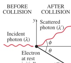
Besides the photoelectric effect, a number of other experiments were carried out in the early twentieth century which also supported the photon theory. One of these was the Compton effect(1923) named after its discoverer, A. H. Compton (1892–1962). Compton aimed short-wavelength light (actually X-rays) at various materials, and detected light scattered at various angles. He found that the scattered light had a slightly longer wavelength than did the incident light, and therefore a slightly lower frequency indicating a loss of energy. He explained this result on the basis of the photon theory as incident photons colliding with electrons of the material, Fig. 27–9. Using Eq. 27–6 for momentum of a photon, Compton applied the laws of conservation of momentum and energy to the collision of Fig. 27–9 and derived the following equation for the wavelength of the scattered photons:

(27;7)

where is the mass of the electron. (The quantity which has the dimen-sions of length, is called the Compton wavelengthof the electron.) We see that the predicted wavelength of scattered photons depends on the angle at which they are detected. Compton’s measurements of 1923 were consistent with this formula. The wave theory of light predicts no such shift: an incoming electro-magnetic wave of frequency fshould set electrons into oscillation at frequency f; and such oscillating electrons would reemit EM waves of this same frequency f (Section 22–2), which would not change with angle Hence the Compton effect adds to the firm experimental foundation for the photon theory of light.

EXERCISE D When a photon scatters off an electron by the Compton effect, which of the following increases: its energy, frequency, wavelength?

X-ray scattering. X-rays of wavelength 0.140 nm are scattered from a very thin slice of carbon. What will be the wavelengths of X-rays scattered at (a) 0°, (b) 90°, (c) 180°?

APPROACH This is an example of the Compton effect, and we use Eq. 27–7 to

find the wavelengths.

SOLUTION (a) For and Then Eq. 27–7

gives This makes sense since for there really isn’t any collision as the photon goes straight through without interacting.

(b) For and So

that is, the wavelength is longer by one Compton wavelength for an electron).

(c) For which means the photon is scattered backward, returning in the direction from which it came (a direct “head-on” collision),

and So

NOTE The maximum shift in wavelength occurs for backward scattering, and it is twice the Compton wavelength.

The Compton effect has been used to diagnose bone disease such as osteoporo-sis. Gamma rays, which are photons of even shorter wavelength than X-rays, coming from a radioactive source are scattered off bone material. The total intensity of the scattered radiation is proportional to the density of electrons, which is in turn proportional to the bone density. A low bone density may indicate osteoporosis.

l¿ = l + 2 h

mec = 0.140nm + 2(0.0024nm) = 0.145nm.

1 - cosf = 2.

cosf = –1, f = 180°,

= 0.0024nm

(= h兾mec2 = 0.140nm + 2.4 * 10–12_{m = 0.142nm;}

l¿ = l + _mh

ec = 0.140nm +

6.63 * 10–34_Js

A9.11 * 10–31_{kgBA3.00 * 10}8_m兾sB

1 - cosf = 1. f = 90°, cosf = 0,

f = 0°, l¿ = l = 0.140nm.

1- cosf = 0. f = 0°, cosf = 1

EXAMPLE 27;8

(f).

f h兾mec,

me

l¿ = l + _mh

ec (1 - cosf),

*

P H Y S I C S A P P L I E D Measuring bone density FIGURE 27–9 The Compton effect. A single photon of wavelength strikes an electron in some material, knocking it out of its atom. The scattered photon has less energy (some energy is given to the electron) and hence has a longer wavelength (shown exaggerated). Experiments found scattered X-rays of just the wavelengths predicted by conservation of energy and

momentum using the photon model.

l¿

l θ

φ

e− Electron at rest initially Incident photon ( )

Scattered photon ( ')

λ

λ

x y

BEFORE COLLISION

27–6

Photon Interactions; Pair Production

1. The photoelectric effect: A photon may knock an electron out of an atom and in the process the photon disappears.

2. The photon may knock an atomic electron to a higher energy state in the atom if its energy is not sufficient to knock the electron out altogether. In this process the photon also disappears, and all its energy is given to the atom. Such an atom is then said to be in an excited state, and we shall discuss it more later. 3. The photon can be scattered from an electron (or a nucleus) and in the

process lose some energy; this is the Compton effect(Fig. 27–9). But notice that the photon is not slowed down. It still travels with speed c, but its frequency will be lower because it has lost some energy.

4. Pair production: A photon can actually create matter, such as the production of an electron and a positron, Fig. 27–10. (A positron has the same mass as an electron, but the opposite charge, )

In process 4, pair production, the photon disappears in the process of creating the electron–positron pair. This is an example of mass being created from pure energy, and it occurs in accord with Einstein’s equation Notice that a photon cannot create an electron alone since electric charge would not then be conserved. The inverse of pair production also occurs: if a positron comes close to an electron, the two quickly annihilate each other and their energy, including their mass, appears as electromagnetic energy of photons. Because positrons are not as plentiful in nature as electrons, they usually do not last long.

Electron–positron annihilation is the basis for the type of medical imaging known as PET, as discussed in Section 31–8.

Pair production. (a) What is the minimum energy of a photon that can produce an electron–positron pair? (b) What is this photon’s wavelength?

APPROACH The minimum photon energy Eequals the rest energy of

the two particles created, via Einstein’s famous equation (Eq. 26–7). There is no energy left over, so the particles produced will have zero kinetic energy. The wavelength is where for the original photon.

SOLUTION (a) Because and the mass created is equal to two electron

masses, the photon must have energy

A photon with less energy cannot undergo pair production.

(b) Since the wavelength of a 1.02-MeV photon is

which is 0.0012 nm. Such photons are in the gamma-ray (or very short X-ray) region of the electromagnetic spectrum (Fig. 22–8).

NOTE Photons of higher energy (shorter wavelength) can also create an electron– positron pair, with the excess energy becoming kinetic energy of the particles.

Pair production cannot occur in empty space, for momentum could not be con-served. In Example 27–9, for instance, energy is conserved, but only enough energy was provided to create the electron–positron pair at rest and thus with zero momen-tum, which could not equal the initial momentum of the photon. Indeed, it can be shown that at any energy, an additional massive object, such as an atomic nucleus (Fig. 27–10), must take part in the interaction to carry off some of the momentum.

l = hc

E =

A6.63 * 10–34_{JsBA3.00 * 10}8_m兾sB

A1.64 * 10–13JB = 1.2 * 10 –12_m,

E = hf = hc兾l,

(1MeV = 106_{eV = 1.60 * 10}–13_J).

E = 2A9.11 * 10–31_{kgBA3.00 * 10}8_m兾sB2 _{= 1.64 * 10}–13_{J = 1.02MeV}

E = mc2_,

E = hf

l = c兾f

E = mc2 Amc

2_B

EXAMPLE 27;9

E = mc2_.

±e.

SECTION 27–6 Photon Interactions; Pair Production

781

e

Nucleus

e− Photon

27–7

Wave–Particle Duality; the

Principle of Complementarity

It is not easy to “visualize” this duality. We cannot readily picture a combina-tion of wave and particle. Instead, we must recognize that the two aspects of light are different “faces” that light shows to experimenters.

Part of the difficulty stems from how we think. Visual pictures (or models) in our minds are based on what we see in the everyday world. We apply the concepts of waves and particles to light because in the macroscopic world we see that energy is transferred from place to place by these two methods. We cannot see directly whether light is a wave or particle, so we do indirect experiments. To explain the experiments, we apply the models of waves or of particles to the nature of light. But these are abstractions of the human mind. When we try to conceive of what light really “is,” we insist on a visual picture. Yet there is no reason why light should conform to these models (or visual images) taken from the macroscopic world. The “true” nature of light—if that means anything—is not possible to visualize. The best we can do is recognize that our knowledge is limited to the indirect experiments, and that in terms of everyday language and images, light reveals both wave and particle properties.

It is worth noting that Einstein’s equation itself links the particle and wave properties of a light beam. In this equation,Erefers to the energy of a particle; and on the other side of the equation, we have the frequency fof the corresponding wave.

27–8

Wave Nature of Matter

In 1923, Louis de Broglie (1892–1987) extended the idea of the wave–particle duality. He appreciated the symmetry in nature, and argued that if light some-times behaves like a wave and somesome-times like a particle, then perhaps those things in nature thought to be particles—such as electrons and other material objects— might also have wave properties. De Broglie proposed that the wavelength of a material particle would be related to its momentum in the same way as for a photon, Eq. 27–6, That is, for a particle having linear momentum

the wavelength is given by

(27;8)

and is valid classically ( for ) and relativistically

This is sometimes called the de Broglie wavelength of a particle.

mv兾₃1 - v2_兾c2_B. Ap =

g_{mv =}

v V c

p = mv

l = h_p,

l p = mv

, p = h兾l.

E = hf

C A U T I O N

Not correct to say light is a wave and/or a particle. Light can actlike a wave or like a particle FIGURE 27–11 Niels Bohr (right), walking with Enrico Fermi along the Appian Way outside Rome. This photo shows one important way physics is done.

Wavelength of a ball. Calculate the de Broglie wavelength of a 0.20-kg ball moving with a speed of

APPROACH We use Eq. 27–8.

SOLUTION

Ordinary objects, such as the ball of Example 27–10, have unimaginably small wavelengths. Even if the speed is extremely small, say the wavelength would be about Indeed, the wavelength of any ordinary object is much too small to be measured and detected. The problem is that the properties of waves, such as interference and diffraction, are significant only when the size of objects or slits is not much larger than the wavelength. And there are no known objects or slits to diffract waves only long, so the wave properties of ordinary objects go undetected.

But tiny elementary particles, such as electrons, are another matter. Since the mass mappears in the denominator of Eq. 27–8, a very small mass should have a much larger wavelength.

Wavelength of an electron. Determine the wavelength of an electron that has been accelerated through a potential difference of 100 V.

APPROACH If the kinetic energy is much less than the rest energy, we can use

the classical formula, (see end of Section 26–9). For an electron, We then apply conservation of energy: the kinetic energy acquired by the electron equals its loss in potential energy. After solving for v, we use Eq. 27–8 to find the de Broglie wavelength.

SOLUTION The gain in kinetic energy equals the loss in potential energy:

Thus so The ratio

so relativity is not needed. Thus

and

Then

or 0.12 nm.

EXERCISE E As a particle travels faster, does its de Broglie wavelength decrease, increase, or remain the same?

EXERCISE F Return to the Chapter-Opening Question, page 771, and answer it again now. Try to explain why you may have answered differently the first time.

Electron Diffraction

From Example 27–11, we see that electrons can have wavelengths on the order of and even smaller. Although small, this wavelength can be detected: the spacing of atoms in a crystal is on the order of and the orderly array of atoms in a crystal could be used as a type of diffraction grating, as was done earlier for X-rays (see Section 25–11). C. J. Davisson and L. H. Germer per-formed the crucial experiment: they scattered electrons from the surface of a metal crystal and, in early 1927, observed that the electrons were scattered into a pattern of regular peaks. When they interpreted these peaks as a diffraction pattern, the wavelength of the diffracted electron wave was found to be just that predicted by de Broglie, Eq. 27–8. In the same year, G. P. Thomson (son of J. J. Thomson) used a different experimental arrangement and also detected diffraction of electrons. (See Fig. 27–12. Compare it to X-ray diffraction, Section 25–11.) Later experiments showed that protons, neutrons, and other particles also have wave properties.

10–10_m

10–10_m,

l = _mvh = A6.63 * 10

–34_JsB

A9.1 * 10–31kgBA5.9 * 106m兾sB = 1.2 * 10 –10_m,

v = _B2_meV = _C(2)A1.6 * 10

–19

CB(100V)

A9.1 * 10–31_kgB = 5.9 * 10 6_m兾s.

1 2mv

2 _{= eV}

100eV兾A0.511 * 106_{eVB L 10}–4_,

ke兾mc2 ₌

ke = 100eV.

ke = eV,

¢pe = eV - 0. mc2 _{= 0.511MeV.}

ke = 1

2mv2

EXAMPLE 27;11

10–30_m

10–29_m.

10–4_m兾s,

l = h_p = _mvh = A6.6 * 10 –34

JsB

(0.20kg)(15m兾s) = 2.2 * 10 –34_m.

15m兾s.

EXAMPLE 27;10

SECTION 27–8 Wave Nature of Matter

783

Thus the wave–particle duality applies to material objects as well as to light. The principle of complementarity applies to matter as well. That is, we must be aware of both the particle and wave aspects in order to have an understanding of matter, including electrons. But again we must recognize that a visual picture of a “wave–particle” is not possible.

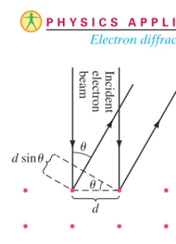
Electron diffraction. The wave nature of electrons is mani-fested in experiments where an electron beam interacts with the atoms on the surface of a solid, especially crystals. By studying the angular distribution of the diffracted electrons, one can indirectly measure the geometrical arrangement of atoms. Assume that the electrons strike perpendicular to the surface of a solid (see Fig. 27–13), and that their energy is low, so that they interact only with the surface layer of atoms. If the smallest angle at which a diffraction maximum occurs is at 24°, what is the separation dbetween the atoms on the surface?

SOLUTION Treating the electrons as waves, we need to determine the

condi-tion where the difference in path traveled by the wave diffracted from adjacent atoms is an integer multiple of the de Broglie wavelength, so that constructive interference occurs. The path length difference is (Fig. 27–13); so for the smallest value of we must have

However, is related to the (non-relativistic) kinetic energy by

Thus

The surface inter-atomic spacing is

NOTE Experiments of this type verify both the wave nature of electrons and the orderly array of atoms in crystalline solids.

What Is an Electron?

We might ask ourselves: “What is an electron?” The early experiments of J. J. Thomson (Section 27–1) indicated a glow in a tube, and that glow moved when a magnetic field was applied. The results of these and other experiments were best interpreted as being caused by tiny negatively charged particles which we now call electrons. No one, however, has actually seen an electron directly. The drawings we sometimes make of electrons as tiny spheres with a negative charge on them are merely convenient pictures (now recognized to be inaccurate). Again we must rely on experimental results, some of which are best interpreted using the particle model and others using the wave model. These models are mere pictures that we use to extrapolate from the macroscopic world to the tiny microscopic world of the atom. And there is no reason to expect that these models somehow reflect the reality of an electron. We thus use a wave or a particle model (whichever works best in a situation) so that we can talk about what is happening. But we should not be led to believe that an electron isa wave or a particle. Instead we could say that an electron is the set of its properties that we can measure. Bertrand Russell said it well when he wrote that an electron is “a logical construction.”

d = l

sinu =

0.123nm

sin 24° = 0.30nm.

= A6.63 * 10

–34_JsB

32A9.11 * 10–31_{kgB(100eV)A1.6 * 10}–19_J兾eVB = 0.123nm.

l = h

32m_eke

ke = p

2

2m_e = h2

2m_el2.

ke l

dsinu = l.

u dsinu

ke = 100eV,

EXAMPLE 27;12 P H Y S I C S A P P L I E D

Electron diffraction

FIGURE 27–13 Example 27–12. The red dots represent atoms in an orderly array in a solid.

d sin u

d

u

u

Incident

electron

27–9

Electron Microscopes

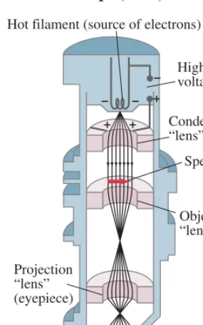
The idea that electrons have wave properties led to the development of the electron microscope(EM), which can produce images of much greater magnifi-cation than a light microscope. Figures 27–14 and 27–15 are diagrams of two types, developed around the middle of the twentieth century: the transmission electron microscope(TEM), which produces a two-dimensional image, and the scanning electron microscope(SEM), which produces images with a three-dimensional quality.

SECTION 27–9

785

FIGURE 27–14 Transmission electron microscope. The magnetic field coils are designed to be “magnetic lenses,” which bend the electron paths and bring them to a focus, as shown. The sensors of the image measure electron intensity only, no color.

+

– +

–

+ –

Hot filament (source of electrons)

High voltage

Condensing “lens”

Specimen

Objective “lens”

Image (on screen, film, or semiconductor detector) Projection

“lens” (eyepiece)

Electron source

Magnetic lens

Electron collector

Electronics and screen

Secondary electrons Specimen

Scanning coils

(a) (b) (c)

FIGURE 27–16 Electron micrographs, in false color, of (a) viruses attacking a cell of the bacterium Escherichia

coli(TEM, (b) Same

subject by an SEM

(c) SEM image of an eye’s retina (Section 25–2); the rods and cones have been colored beige and green, respectively. Part (c) is also on the cover of this book.

(L35,000*). L50,000*).

In both types, the objective and eyepiece lenses are actually magnetic fields that exert forces on the electrons to bring them to a focus. The fields are produced by carefully designed current-carrying coils of wire. Photographs using each type are shown in Fig. 27–16. EMs measure the intensity of electrons, producing mono-chromatic photos. Color is often added artificially to highlight.

As discussed in Sections 25–7 and 25–8, the maximum resolution of details on an object is about the size of the wavelength of the radiation used to view it. Electrons accelerated by voltages on the order of have wavelengths of about 0.004 nm. The maximum resolution obtainable would be on this order, but in practice, aberrations in the magnetic lenses limit the resolution in transmission electron microscopes to about 0.1 to 0.5 nm. This is still 1000 times better than a visible-light microscope, and corresponds to a useful magnification of about a million. Such magnifications are difficult to achieve, and more common magnifi-cations are to The maximum resolution of a scanning electron microscope is less, typically 5 to 10 nm although new high-resolution SEMs approach 1 nm.

105_.

104

105_V

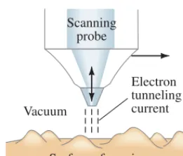
The scanning tunneling electron microscope(STM), developed in the 1980s, contains a tiny probe, whose tip may be only one (or a few) atoms wide, that is moved across the specimen to be examined in a series of linear passes. The tip, as it scans, remains very close to the surface of the specimen, about 1 nm above it, Fig. 27–17. A small voltage applied between the probe and the surface causes electrons to leave the surface and pass through the vacuum to the probe, by a process known as tunneling (discussed in Section 30–12). This “tunneling” current is very sensitive to the gap width, so a feedback mechanism can be used to raise and lower the probe to maintain a constant electron current. The probe’s vertical motion, following the surface of the specimen, is then plotted as a function of position, scan after scan, producing a three-dimensional image of the surface. Surface features as fine as the size of an atom can be resolved: a resolu-tion better than 50 pm (0.05 nm) laterally and 0.01 to 0.001 nm vertically. This kind of resolution has given a great impetus to the study of the surface structure of materials. The “topographic” image of a surface actually represents the distribution of electron charge.

The atomic force microscope (AFM), developed in the 1980s, is in many ways similar to an STM, but can be used on a wider range of sample materials. Instead of detecting an electric current, the AFM measures the force between a cantilevered tip and the sample, a force which depends strongly on the tip–sample separation at each point. The tip is moved as for the STM.

27–10

Early Models of the Atom

The idea that matter is made up of atoms was accepted by most scientists by 1900. With the discovery of the electron in the 1890s, scientists began to think of the atom itself as having a structure with electrons as part of that structure. We now discuss how our modern view of the atom developed, and the quantum theory with which it is intertwined.†

A typical model of the atom in the 1890s visualized the atom as a homogene-ous sphere of positive charge inside of which there were tiny negatively charged electrons, a little like plums in a pudding, Fig. 27–18.

Around 1911, Ernest Rutherford (1871–1937) and his colleagues performed experiments whose results contradicted the plum-pudding model of the atom. In these experiments a beam of positively charged alpha particles was directed at a thin sheet of metal foil such as gold, Fig. 27–19. (These newly discovered

particles were emitted by certain radioactive materials and were soon shown to be doubly ionized helium atoms—that is, having a charge of ±2e.) It was a

(a) P H Y S I C S A P P L I E D

STM and AFM

FIGURE 27–17 The probe tip of a scanning tunneling electron microscope, as it is moved

horizontally, automatically moves up and down to maintain a constant tunneling current, and this motion is translated into an image of the surface.

Vacuum

Electron tunneling current

Surface of specimen Scanning

probe

FIGURE 27–18 Plum-pudding model of the atom.

Positively charged material

– –

– –

– –

≈10−10m

FIGURE 27–19 Experimental setup for Rutherford’s experiment:

particles emitted by radon are deflected by the atoms of a thin metal foil and a few rebound backward.

a

Viewing screen

Source containing radon

particles

Metal foil

†_{Some readers may say: “Tell us the facts as we know them today, and don’t bother us with the}

histor-ical background and its outmoded theories.” Such an approach would ignore the creative aspect of science and thus give a false impression of how science develops. Moreover, it is not really possible to understand today’s view of the atom without insight into the concepts that led to it.

And of those deflected, a few were deflected at very large angles—some even backward, nearly in the direction from which they had come. This could happen, Rutherford reasoned, only if the positively charged alpha particles were being repelled by a massive positive charge concentrated in a very small region of space (see Fig. 27–20). He hypothesized that the atom must consist of a tiny but mas-sive positively charged nucleus, containing over 99.9%of the mass of the atom, surrounded by much lighter electrons some distance away. The electrons would be moving in orbits about the nucleus—much as the planets move around the Sun—because if they were at rest, they would fall into the nucleus due to electri-cal attraction. See Fig. 27–21. Rutherford’s experiments suggested that the nucleus must have a radius of about to From kinetic theory, and especially Einstein’s analysis of Brownian motion (see Section 13–1), the radius of atoms was estimated to be about Thus the electrons would seem to be at a distance from the nucleus of about 10,000 to 100,000 times the radius of the nucleus itself. (If the nucleus were the size of a baseball, the atom would have the diameter of a big city several kilometers across.) So an atom would be mostly empty space.

Rutherford’s planetary model of the atom (also called the nuclear model of the atom) was a major step toward how we view the atom today. It was not, however, a complete model and presented some major problems, as we shall see.

27–11

Atomic Spectra: Key to the

Structure of the Atom

Earlier in this Chapter we saw that heated solids (as well as liquids and dense gases) emit light with a continuous spectrum of wavelengths. This radiation is assumed to be due to oscillations of atoms and molecules, which are largely governed by the interaction of each atom or molecule with its neighbors.

Rarefied gases can also be excited to emit light. This is done by intense heating, or more commonly by applying a high voltage to a “discharge tube” containing the gas at low pressure, Fig. 27–22. The radiation from excited gases had been observed early in the nineteenth century, and it was found that the spectrum was not continuous. Rather, excited gases emit light of only certain wavelengths, and when this light is analyzed through the slit of a spectroscope or spectrometer, a line spectrum is seen rather than a continuous spectrum. The line spectra emitted by a number of elements in the visible region are shown below in Fig. 27–23, and in Chapter 24, Fig. 24–28. The emission spectrumis characteristic of the material and can serve as a type of “fingerprint” for identification of the gas.

We also saw (Chapter 24) that if a continuous spectrum passes through a rarefied gas, dark lines are observed in the emerging spectrum, at wavelengths corresponding to lines normally emitted by the gas. This is called an absorption spectrum (Fig. 27–23c), and it became clear that gases can absorb light at the same frequencies at which they emit. Using film sensitive to ultraviolet and to infrared light, it was found that gases emit and absorb discrete frequencies in these regions as well as in the visible.

10–10_m.

10–14_m.

10–15

SECTION 27–11 Atomic Spectra: Key to the Structure of the Atom

787

≈10−10_m 10−15_m

–

+

FIGURE 27–22 Gas-discharge tube: (a) diagram; (b) photo of an actual discharge tube for hydrogen.

Anode

High voltage

Cathode

– +

(a)

(b)

+ –

– –

FIGURE 27–23 Emission spectra of the gases (a) atomic hydrogen, (b) helium, and (c) the solar absorptionspectrum.

(a)

(b)

(c)

Nucleus

particle + +

FIGURE 27–20 Backward rebound of particles in Fig. 27–19 explained as the repulsion from a heavy positively charged nucleus.

In low-density gases, the atoms are far apart on average and hence the light emitted or absorbed is assumed to be by individual atomsrather than through interactions between atoms, as in a solid, liquid, or dense gas. Thus the line spectra serve as a key to the structure of the atom: any theory of atomic structure must be able to explain why atoms emit light only of discrete wavelengths, and it should be able to predict what these wavelengths are.

Hydrogen is the simplest atom—it has only one electron orbiting its nucleus. It also has the simplest spectrum. The spectrum of most atoms shows little apparent regularity. But the spacing between lines in the hydrogen spectrum decreases in a regular way, Fig. 27–24. Indeed, in 1885, J. J. Balmer (1825–1898) showed that the four lines in the visible portion of the hydrogen spectrum (with measured wavelengths 656 nm, 486 nm, 434 nm, and 410 nm) have wavelengths that fit the formula

(27;9)

Herentakes on the values 3, 4, 5, 6 for the four visible lines, and R, called the Rydberg constant, has the value Later it was found that thisBalmer seriesof lines extended into the UV region, ending at

as shown in Fig. 27–24. Balmer’s formula, Eq. 27–9, also worked for these lines with higher integer values of n. The lines near 365 nm become too close together to distinguish, but the limit of the series at 365 nm corresponds to (so

in Eq. 27–9).

Later experiments on hydrogen showed that there were similar series of lines in the UV and IR regions, and each series had a pattern just like the Balmer series, but at different wavelengths, Fig. 27–25. Each of these series was found to

1兾n2 _{= 0} n = q

l = 365nm, R = 1.0974 * 107_m–1_.

1

l = R¢ 1 22

-1

n2≤,

FIGURE 27–24 Balmer series of lines for hydrogen.

(nm) 365

410

434

486

Violet

Blue

Blue-green UV

Red 656

λ

Lyman series

UV Visible light IR

Balmer series Paschen series

91 nm 122 nm 365 nm 656 nm 820 nm 1875 nm

Wavelength, λ FIGURE 27–25 Line spectrum of

atomic hydrogen. Each series fits the

formula where

for the Lyman series, for the Balmer series, for the Paschen series, and so on;ncan take on all integer values from up to infinity. The only lines in the visible region of the electromagnetic spectrum are part of the Balmer series.

n = n¿ +1 n¿ = 3

n¿ = 2 n¿ = 1

1

l = R¢

1 nœ2

-1 n2≤

fit a formula with the same form as Eq. 27–9 but with the replaced by and so on. For example, the Lyman series contains lines with wavelengths from 91 nm to 122 nm (in the UV region) and fits the formula

The wavelengths of the Paschen series(in the IR region) fit

The Rutherford model was unable to explain why atoms emit line spectra. It had other difficulties as well. According to the Rutherford model, electrons orbit the nucleus, and since their paths are curved the electrons are accelerating. Hence they should give off light like any other accelerating electric charge (Chapter 22).

1

l = R¢ 1 32

-1

n2≤,

1

l = R¢ 1 12

-1

n2≤,

1兾12_{, 1兾3}2_{, 1兾4}2_,

Since light carries off energy and energy is conserved, the electron’s own energy must decrease to compensate. Hence electrons would be expected to spiral into the nucleus. As they spiraled inward, their frequency would increase in a short time and so too would the frequency of the light emitted. Thus the two main difficulties of the Rutherford model are these: (1) it predicts that light of a continuous range of frequencies will be emitted, whereas experiment shows line spectra; (2) it predicts that atoms are unstable—electrons would quickly spiral into the nucleus—but we know that atoms in general are stable, because there is stable matter all around us. Clearly Rutherford’s model was not sufficient. Some sort of modification was needed, and Niels Bohr provided it in a model that included the quantum hypothesis. Although the Bohr model has been superseded, it did provide a crucial stepping stone to our present understanding. And some aspects of the Bohr model are still useful today, so we examine it in detail in the next Section.

27–12

The Bohr Model

Bohr had studied in Rutherford’s laboratory for several months in 1912 and was convinced that Rutherford’s planetary model of the atom had validity. But in order to make it work, he felt that the newly developing quantum theory would somehow have to be incorporated in it. The work of Planck and Einstein had shown that in heated solids, the energy of oscillating electric charges must change discontinuously—from one discrete energy state to another, with the emission of a quantum of light. Perhaps, Bohr argued, the electrons in an atom also cannot lose energy continuously, but must do so in quantum “jumps.” In working out his model during the next year, Bohr postulated that electrons move about the nucleus in circular orbits, but that only certain orbits are allowed. He further postulated that an electron in each orbit would have a definite energy and would move in the orbit without radiating energy (even though this violated classical ideas since accelerating electric charges are supposed to emit EM waves; see Chapter 22). He thus called the possible orbits stationary states. In this Bohr model, light is emitted only when an electron jumps from a higher (upper) stationary state to another of lower energy, Fig. 27–26. When such a transition occurs, a single pho-ton of light is emitted whose energy, by energy conservation, is given by

(27;10)

where refers to the energy of the upper state and the energy of the lower state.

In 1912–13, Bohr set out to determine what energies these orbits would have in the simplest atom, hydrogen; the spectrum of light emitted could then be pre-dicted from Eq. 27–10. In the Balmer formula he had the key he was looking for. Bohr quickly found that his theory would agree with the Balmer formula if he assumed that the electron’s angular momentum Lis quantized and equal to an integern times As we saw in Chapter 8 angular momentum is given by whereIis the moment of inertia and is the angular velocity. For a single particle of mass mmoving in a circle of radius rwith speed v, and

hence, Bohr’s quantum conditionis

(27;11)

wherenis an integer and is the radius of the nth_{possible orbit. The allowed} orbits are numbered according to the value of n, which is called the principal quantum numberof the orbit.

Equation 27–11 did not have a firm theoretical foundation. Bohr had searched for some “quantum condition,” and such tries as (where Erepresents the energy of the electron in an orbit) did not give results in accord with experi-ment. Bohr’s reason for using Eq. 27–11 was simply that it worked; and we now look at how. In particular, let us determine what the Bohr theory predicts for the measurable wavelengths of emitted light.

E = hf

1, 2, 3, p , rn

L = mvrn = n h

2p,

v = v兾r;

I = mr2

v L = Iv,

h兾2p.

El Eu

hf = Eu - El,

SECTION 27–12 The Bohr Model

789

photon when its

energy changes from to a lower energyE_l.

Eu (energy = hf)

An electron in a circular orbit of radius r(Fig. 27–27) would have a centripetal acceleration produced by the electrical force of attraction between the negative electron and the positive nucleus. This force is given by Coulomb’s law,