Doctoral School in Mathematics
A holistic multi-scale mathematical model of the murine
extracellular fluid systems and study of the brain
interactive dynamics
Christian Contarino
Doctoral thesis in
Mathematics
, XXX cycle
Department of Mathematics,
University of Trento
Academic year: 2016/2017
Supervisor:
Prof. Eleuterio F. Toro
,
University of Trento, Italy
External examiner:
Prof. Vartan Kurtcuoglu
,
University of Zürich, Switzerland
External examiner:
Prof. Roxana O. Carare
,
University of Southampton,
Eng-land
University of Trento
Trento, Italy
If you can dream it, you can do it.
If you can dream it, you can do it.
Walt Disney
Abstract
Recent advances in medical science regarding the interaction and functional role
of fluid compartments in the central nervous system have attracted the attention of
many researchers across various disciplines. Neurotoxins are constantly cleared
from the brain parenchyma through the intramural periarterial drainage system,
glymphatic system and meningeal lymphatic system. Impairment of these systems
can potentially contribute to the onset of neurological disorders.
The goal of this thesis is to contribute to the understanding of brain fluid
dynamics and to the role of vascular pathologies in the context of neurological
disorders. To achieve this goal, we designed the first multi-scale, closed-loop
mathematical model of the murine fluid system, incorporating: heart dynamics,
major arteries and veins, microcirculation, pulmonary circulation, venous valves,
cerebrospinal fluid (CSF), brain interstitial fluid (ISF), Starling resistors,
Monro-Kellie hypothesis, brain lymphatic drainage and the modern concept of CSF/ISF
drainage and absorption based on the
Bulat-Klarica-Orešković
hypothesis. The
mathematical model relies on one-dimensional Partial Differential Equations
(PDEs) for blood vessels and on Ordinary Differential Equations (ODEs) for
lumped parameter models. The systems of PDEs and ODEs are solved through
a high-order finite volume ADER method and through an implicit Euler method.
The computational results are validated against literature values and magnetic
resonance flow measurements. Furthermore, the model is validated against
in-vivo
intracranial pressure waveforms acquired in healthy mice and in mice with
impairment of the intracranial venous outflow. Through a systematic use of our
computational model in healthy and pathological cases, we provide a complete
and holistic neurovascular view of the main murine fluid dynamics. We propose
a hypothesis on the working principles of the glymphatic system, opening a
new door towards a comprehensive understanding of the mechanisms which link
vascular and neurological disorders. In particular, we show how impairment of
the cerebral venous outflow might potentially lead to accumulation of solutes in
the parenchyma, by altering CSF and ISF dynamics.
Preface
The research of this PhD thesis was carried out in the Department of
Math-ematics of the University of Trento under the supervision of Prof. Eleuterio F.
Toro.
I sincerely thank Prof. J. Kipnis (Department of Neuroscience, University of
Virginia, Charlottesville, USA) for the opportunity he gave me to visit his lab.
I sincerely thank Prof. E. M. Haacke (MR Research Facility, Wayne State
University, Detroit, USA) for providing the software SPIN (Signal Processing in
NMR, Detroit, MI) for blood and CSF MR-flow analysis.
In Chapter
4
, Dr. I. Smirnov conducted the surgery and interventions, Dr. A.
Louveau acquired the intracranial measurements.
Acknowledgements
During the PhD journey, I encountered many challenges from both scientific and family
point of views. Probably, the PhD journey has been one of the most significant experiences
that allowed me to grow as a person and as a scientist. Nothing would have been possible
without the help and support of many people I met during these three significant years.
Every person, every chat, every moment of sharing allowed me to move forward and dream
the life dream.
Nothing would have been possible without my family, from Danilo to my mother and
father. You all believed, supported me and made many sacrifices to allow me to continue
studying. Danilo, you are my supporting pillar and helped me in the most difficult situations.
My mother taught me how important sacrifice is and what unlimited love is. My father
taught me how to be strong and endure difficult situations.
I will always be grateful to my supervisor, Prof. Eleuterio F. Toro. You taught me the
enthusiasm for research, believed in me, guided me through the PhD journey and changed
my life several times. A wholehearted
thank
.
I will always be grateful to Dr Nivedita Agarwal. You taught me that we always have
to fight for what we believe in and that nothing can stop us.
I will always be grateful to Federica Caforio. You taught me to never give up, that there
will be always the third solution in the most difficult moments.
I will always be grateful to Simona Biancheri. You taught me how powerful words can
be and you trusted me beyond the limits of life.
I wish to thank all fellows at the Department of Neuroscience of the University of
Vir-ginia in Charlottesville and all fellows at the Department of Mathematics of the University
of Trento in Italy. I wish to thank all of my friends who believed in me and laughed with
me even with the useless game "ce l’hai" which however has the incredible power to give a
smile.
Thanks
.
I also thank the University of Trento, and in particular the Department of Mathematics,
for providing the funding and the academic support to carry out my research. I wish to
thank all professors at the University of Trento, in particular, Prof. Alberto Valli and Prof.
Ana Alonso Rodriguez.
Contents
Abstract vii
Preface ix
Acknowledgements xi
Contents xv
List of Figures xviii
List of Tables xix
Papers published or submitted during the PhD candidature xxi
Conference presentations during the PhD candidature xxiii
1 Introduction 1
1.1 Motivation and goals. . . 1
1.2 State of the art . . . 2
1.2.1 The vascular system. . . 2
1.2.2 The brain fluid systems . . . 3
1.2.3 The lymphatic system . . . 3
1.2.4 High-order numerical methods for partial differential equations . . . 4
1.3 Contributions of this thesis . . . 4
2 Junction-generalized Riemann problem for stiff hyperbolic balance laws in networks: An implicit solver and ADER schemes 7 2.1 Introduction . . . 7
2.2 Methods . . . 9
2.2.1 One-dimensional blood flow equations . . . 9
2.2.2 ADER finite volume scheme . . . 11
2.2.3 The Junction-Generalized Riemann Problem (J-GRP) . . . 15
2.2.4 A new implicit J-GRP solver . . . 21
2.3 Results . . . 24
2.3.1 Empirical convergence rate studies . . . 25
2.3.2 A stiff problem for a junction . . . 29
2.3.3 Application to a network of arteries. . . 32
2.4 Summary and conclusions . . . 39
3 A one-dimensional mathematical model of collecting lymphatics coupled with an
electro-fluid-mechanical contraction model and valve dynamics 41
3.1 Introduction . . . 41
3.2 Methods . . . 43
3.2.1 A one-dimensional model for lymph flow . . . 43
3.2.2 The Electro-Fluid-Mechanical Contraction (EFMC) model . . . 48
3.2.3 A lumped-parameter model for lymphatic valves . . . 54
3.2.4 Numerical methods . . . 55
3.2.5 Sensitivity Analysis . . . 60
3.3 Results . . . 61
3.3.1 Test problem with piecewise initial condition: a Riemann problem. . . 61
3.3.2 Representative test problems for lymphatic vessels. . . 62
3.3.3 Pressure versus normalised cross-sectional area (PA) plots for a single lym-phangion . . . 68
3.3.4 Analysis of lymphatic indices by varyingPinandPout . . . 68
3.3.5 Sensitivity analyses of the mathematical model. . . 74
3.3.6 A quantitative study on the effect of stenotic and regurgitant lymphatic valves 74 3.4 Discussion . . . 78
3.4.1 Comparison between zero and one-dimensional models . . . 78
3.4.2 Characterization of the lymphatic wall electrical activity . . . 78
3.4.3 Frequency of contractions of the EFMC depend on local fluid dynamics . . . 79
3.4.4 The advantage of the EFMC model in networks of collecting lymphatics . . . 79
3.4.5 Extension of the Mynard’s valve model to the lymphatic framework . . . 79
3.4.6 A theoretical study of lymphatic valve impairments. . . 80
3.5 Limitations and future development . . . 80
3.6 Conclusion . . . 81
4 Working principles of the glymphatic system: A hypothesis based on a holistic multi-scale mathematical model of the murine extracellular fluid systems 83 4.1 Introduction . . . 83
4.2 Methods . . . 84
4.2.1 One-dimensional blood flow equations . . . 89
4.2.2 Zero-dimensional mathematical models. . . 91
4.2.3 Numerical methods for the solution of the system of equations. . . 111
4.2.4 In-vivomagnetic resonance imaging in mice: angiography, venography and blood flow quantification . . . 112
4.2.5 In-vivointracranial pressure measurements . . . 113
4.2.6 Allometric scaling: from humans to mice . . . 114
4.3 Results . . . 114
4.3.1 Validation of the computational results againstin-vivomeasurements. . . 119
4.3.2 Dynamics of heart and peripheral vascular system . . . 122
4.3.3 Dynamics of intracranial blood vessels . . . 122
4.3.4 Cerebrospinal fluid dynamics and its interaction with intracranial blood . . . 123
4.3.5 Interaction of heart, brain interstitial fluid and cerebrospinal fluid and the regulation of brain fluids . . . 123
4.3.6 Alteration of CSF absorption, Starling forces, ISF-CSF permeability and the Monro-Kellie coupling: a mathematical study of the intracranial effect . . . . 129
4.3.7 Idiopathic intracranial hypertension and CSF-ISF alterations . . . 131
CONTENTS
xv
4.4.1 Mathematical models of the main murine fluid systems and comparison with
the body of literature . . . 133
4.4.2 Intraparenchymal bidirectional water movement: the heart influence . . . 134
4.4.3 Brain fluid homeostasis: modern view of CSF drainage . . . 134
4.4.4 A hypothesis on the working principles of the glymphatic system . . . 135
4.4.5 Alterations of CSF absorption, ISF-CSF permeability, Monro-Kellie coupling and Starling forces affect the glymphatic system . . . 136
4.4.6 Impairment of intracranial venous outflow affects the glymphatic system . . . 137
4.5 Conclusions . . . 139
4.6 Limitations and future development . . . 139
5 Conclusions 141 5.1 Achievements . . . 141
5.1.1 Insights into the glymphatic system and murine fluid dynamics . . . 141
5.1.2 Towards a multi-scale mathematical model for the human lymphatic system . 141 5.1.3 High-order methods for networks of one-dimensional subdomains . . . 142
5.2 Future work . . . 142
List of Figures
2.1 Illustration of an initial condition for a J-GRP. . . 16
2.2 Representation of a J-CRP for a typical2×2non-linear system with N=3vessels. 18 2.3 Example of a J-CRP. . . 19
2.4 Illustration of the MT-HEOC solver for the J-GRP withN=3 vessels.. . . 21
2.5 Three-vessel J-GRP using the MT-HEOC solver. . . 23
2.6 Efficiency plot: L∞ errors against computational times. . . 25
2.7 Illustration of the empirical convergence rate study.. . . 27
2.8 A stiff problem connecting three vessels at a single junction. . . 30
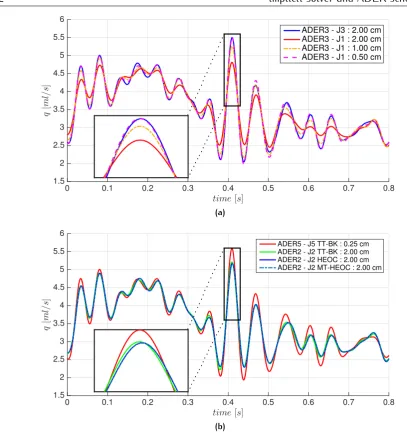
2.9 Computed flow q(x,t)at midpoint of left renal artery, comparing fully and partially fourth-order methods with different mesh sizes. . . 31
2.10 Computed flow q(x,t)at midpoint of left renal artery, comparing fully and partially second-order methods with different mesh sizes.. . . 32
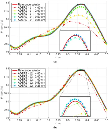
2.11 Computed pressure along the aorta and part of the right iliac femoral, fully and partially second-order ADER schemes. . . 33
2.12 Computed pressure along the aorta and part of the right iliac femoral, fully and partially third-order ADER schemes. . . 34
2.13 Computed pressure along the aorta and part of the right iliac femoral, fully and partially fourth-order ADER schemes.. . . 35
2.14 Computed pressure along the aorta and part of the right iliac femoral, fully and partially second-order ADER schemes with a minimum number of 5 cells.. . . 36
2.15 Efficiency plot for a network of arteries: L1 errors against computational times. . . . 39
3.1 Illustration of a collecting lymphatic. . . 43
3.2 Pressure-diameter relation (tube law). . . 45
3.3 Stability analysis of the stationary point (0,0) of the modified FitzHugh-Nagumo model. . . 49
3.4 Illustration of the EFMC model in the time domain of two representative lymphatic cycles. . . 51
3.5 Illustration of the EFMC model in phase space of a representative lymphatic cycle. . 52
3.6 Effects of EFMC model parameters on the pressure-frequency and WSS-frequency relationships. . . 53
3.7 Framework for a finite volume scheme. . . 56
3.8 Illustration of the coupling method between two lymphangions and one valve. . . 57
3.9 Riemann problem for a single lymphangion without contractions. . . 61
3.10 Test 1: representative case of a single lymphangion. . . 63
3.11 Test 1: representative case of a single lymphangion (space-time). . . 64
3.12 Test 2: contraction frequency increases as the intraluminal pressure increases. . . . 65
3.13 Test 3: contraction frequency decreases with increasing WSS. . . 67
3.14 Transmural pressure against normalised cross-sectional area (PA) plots during lym-phatic contractions . . . 70
3.15 Counterplots of lymphatic indices in thePin−Pout plane. . . 71
3.16 Effect of stenotic and regurgitant lymphatic valves. . . 75
3.17 High frequencies of contractions with a left stenotic valve diminish the CPF. . . 76
4.1 Modelling network of the murine arterial tree. . . 85
4.2 Modelling network of the murine arterial tree (head and neck). . . 86
4.3 Modelling network of the murine venous tree. . . 87
4.4 Modelling network of the murine venous tree (head and neck). . . 88
4.5 Framework for a finite volume scheme. . . 111
4.6 MRI segmentation of murine arterial and venous systems. . . 119
4.7 MRI segmentation of murine brain ventricular, arterial and venous systems. . . 120
4.8 MRI segmentation of murine brain ventricular structure. . . 121
4.9 Validation of computational results againstin-vivoflow and pressure measurements. 124 4.10 Computational results for heart, pulmonary circulation, major arteries and veins. . . . 125
4.11 Computational results of brain blood fluid dynamics. . . 126
4.12 Interactive dynamics of cerebrospinal fluid, arterial and venous blood. . . 127
4.13 Dynamics of cerebrospinal fluid and brain interstitial fluid. . . 128
4.14 Alterations of CSF absorption, Starling forces, ISF-CSF permeability and the Monro-Kellie coupling affect the glymphatic function. . . 130
4.15 Cerebral venous outflow impairment alters the intracranial fluid dynamics. . . 132
List of Tables
2.1 Convergence rates study. . . 26
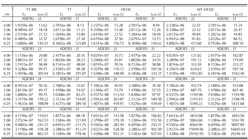
2.2 Errors and computational times for a network of arteries. . . 38
3.1 Parameters used for the one-dimensional EFMC model for lymph flow. . . 46
3.2 Lymphatic indices. . . 69
3.3 Sensitivity analysis of the one-dimensional lymph flow equations coupled to the EFMC model and valve dynamics. Adverse pressure difference case.. . . 72
3.4 Sensitivity analysis of the one-dimensional lymph flow equations coupled to the EFMC model and valve dynamics. Favourable pressure difference case. . . 73
3.5 Analysis of the effect of lymphatic valve deficits.. . . 77
4.1 Geometrical and mechanical parameters for the modelled venous and arterial systems.101 4.2 Parameters for zero-dimensional models. . . 104
4.3 Parameters for zero-dimensional flow dynamics. . . 109
4.4 Parameters for cardiac model, venous valve dynamics and blood rheology. . . 110
4.5 Validation of the computational results. . . 118
Papers published or submitted during the PhD candidature
• E. F. Toro, F. Borgioli, Q. Zhang, C. Contarino, L. O. Mueller and A. Bruno, "Inner-ear cir-culation in humans is disrupted by extracranial venous outflow strictures: Implications for
Ménière’s disease",Veins and Lymphatics, 7 (2018): 10-21.
• C. Contarino, E. F. Toro, G. Montecinos, J. Kall and R. Borsche,"Junction-generalized Riemann
problem for stiff hyperbolic balance laws in networks: An implicit solver and ADER schemes",
Journal of Computational Physics, 315 (2016): 409-433.
• M. Strocchi, C. Contarino, Q. Zhang, E. F. Toro and R. Bonmassari, "A global mathematical
model for the simulation of stenoses and bypass placement in the human arterial system",
Applied Mathematics and Computation, 300 (2017): 21–39.
• C. Spiller, E. F. Toro, M. E. Vazquez and C. Contarino, "On the exact solution of the
Rie-mann problem for blood flow in human veins, including collapse",Applied Mathematics and
Computation, 303 (2017): 178–189.
• S. Da Mesquita, A. Louveau, A. Vaccari, I. Smirnov, R. C. Cornelison, K. M. Kingsmore, C. Contarino, S. Onengut-Gumuscu, E. Farber, D. Raper, K. E. Var, W. Baker, N. Dabhi, G. Oliver, S. Rich, J. M. Munson, C. C. Overall, S. T. Acton and J. Kipnis,"CNS-draining
lymphat-ics play a key role in age-dependent cognitive decline and Alzheimer’s disease pathology",
Nature, Under review (2018).
• C. Contarino and E. F. Toro,"A one-dimensional mathematical model of collecting lymphatics
coupled with an electro-fluid-mechanical contraction model and valve dynamics",
Biomechan-ics and Modelling in Mechanobiology, Under review (2018).
• N. Agarwal, C. Contarino, G. Rossi, C. Stegagno, L. Bertolasi and E. F. Toro, "Intracranial
fluid dynamics changes in idiopathic intracranial hypertension: pre and post therapy",Current
Neurovascular Research, In press (2018).
• E. F. Toro, B. Thornber, Q. Zhang and C. Contarino,"A one-dimensional computational model
of the spinal cerebrospinal fluid", Journal of Biomechanical Engineering, Under review
(2018).
Conference presentations during the PhD candidature
• C. Contarino, E. F. Toro, A. Louveau, S. Da Mesquita, D. Raper, I. Smirnov, N. Agarwal and J. Kipnis,"The role of water dynamics in the glymphatic system through a holistic multi-scale
mathematical model of the murine extracellular fluid systems",Società Italiana di Matematica
Applicata e Industriale (SIMAI) (scheduled) 2018, Rome, Italy.
• C. Contarino, E. F. Toro, A. Louveau, S. Da Mesquita, D. Raper, I. Smirnov, N. Agarwal and J. Kipnis,"A holistic multi-scale mathematical model of the murine fluid systems: understanding
the pathophysiology of idiopathic intracranial hypertension", International Association for
Hydro-Environment Engineering and Research (IAHR) (scheduled) 2018, Trento, Italy.
• C. Contarino, E. F. Toro, A. Louveau, S. Da Mesquita, D. Raper, I. Smirnov, N. Agarwal and J. Kipnis,"A global, multi-scale mathematical model of the murine fluid systems: Application
to idiopathic intracranial hypertension", Istituto Nazionale di Alta Matematica (INdAM)
Workshop 2018, Rome, Italy.
• C. Contarino and E. F. Toro,"Modelling the lymphatics: A 1D lymph flow model coupled to an
electro-fluid-mechanical contraction model", Computational and Mathematical Biomedical
Engineering (CMBE) 2017, Pittsburgh, United States.
• B. Thornber, Q. Zhang, C. Contarino and E. F. Toro,"A one-dimensional computational model
of the spinal cerebrospinal fluid",Computational and Mathematical Biomedical Engineering
(CMBE) 2017, Pittsburgh, United States.
• C. Contarino and E. F. Toro,"A one-dimensional mathematical model for dynamically
contract-ing collectcontract-ing lymphatics",Società Italiana di Matematica Applicata e Industriale (SIMAI)
2016, Milan, Italy.
• C. Contarino, E. F. Toro, G. I. Montecinos, R. Borsche and J. Kall, "Junction-generalized
Riemann problem for stiff hyperbolic balance laws in networks of blood vessels", Società
Italiana di Matematica Applicata e Industriale (SIMAI) 2016, Milan, Italy.
• C. Contarino, E. F. Toro, G. I. Montecinos, R. Borsche and J. Kall, "Junction-generalized
Riemann problem for stiff hyperbolic balance laws in networks of blood vessels",Platform for
Advanced Scientific Computing (PASC) 2016, Lausanne, Switzerland.
• C. Contarino and E. F. Toro,"A first step towards a mathematical model for the human
lym-phatic system",International Society for Neurovascular Disease (ISNVD) 2016, New York,
United States.
• C. Contarino, Q. Zhang, E. F. Toro and G. I. Montecinos,"A first step towards a mathematical
model for the human lymphatic system", European Workshop on High Order Nonlinear
Numerical Methods for Evolutionary PDEs: Theory and Applications (HONOM) 2015, Trento, Italy.
• C. Contarino, Q. Zhang, E. F. Toro and G. I. Montecinos, "Towards high-order methods for
blood flow",Computational and Mathematical Biomedical Engineering (CMBE) 2015,
San-cha, France.
Chapter 1
Introduction
1.1
Motivation and goals
In recent years, there have been several fundamental discoveries that have brought a lot of excite-ment in the field of neurological disorders. The meningeal lymphatic system is a complex network of lymphatic vessels which mainly drains immune cells and cerebrospinal fluid and is a key compo-nent of brain homeostasis [Louveau 2015,Louveau 2017,Absinta 2017]. Brain interstitial fluid and amyloid β drain from the parenchyma along the basement membranes of capillaries and arteries
through intramural periarterial drainage pathways [Carare 2008]. Also, it has been shown that the brain is constantly cleared from neurotoxins through the so-called glymphatic system [Iliff 2012]. The glymphatic system consists of a trans-parenchymal cerebrospinal fluid (CSF) movement through glial cells from para-arterial CSF spaces to para-venous CSF spaces. Intracranial solutes and waste products are transported through the trans-parenchymal water movement towards para-venous CSF spaces and are drained into the venous system through arachnoid villi or meningeal lymphatics
[Louveau 2017]. Thanks to this pseudolymphatic function of waste removal and to the trans-glial
water movement, this system has been termed "glymphatic system". Impairment of the glymphatic system seems to correlate with amyloid β accumulation, a characteristic hallmark of Alzheimer’s
disease [Iliff 2012,Iliff 2014], with migraine [Schain 2017], and idiopathic intracranial hypertension [Bezerra 2018].
Despite the importance of the glymphatic system, it is not yet clear what are its driving forces. Originally, it was proposed that the glymphatic system was driven by bulk flow [Iliff 2012] and arterial pulsations [Iliff 2013]. In general, three possible mechanisms have been proposed: diffu-sion, advection (or bulk flow), and convection defined as a combination of diffusion and advection [Plog 2018]. In contrast with the original idea of Iliff et al. [Iliff 2013], Asgari et al. [Asgari 2016] showed through computational simulations that arterial pulsation is probably not the driving force of the glymphatic system. Also, Smith et al. [Smith 2017] showed that the glymphatic system is unlikely driven by bulk flows. Their results suggest that water movement in the cranial subarach-noid space is driven by convection, while that within the parenchyma is driven by diffusion. To date, however, there is not yet a conclusive explanation of the mechanisms which drive the glymphatic system.
Neurological disorders have been shown to correlate with vascular diseases. Zamboni et al.
[Zamboni 2008] described the so-called Chronic Cerebro-Spinal Venous Insufficiency (CCSVI) and suggested that it is associated with multiple sclerosis. The CCSVI is a condition characterized by obstructed blood flow in the major veins that drain the central nervous system and by iron accumulation [Singh 2009]. Although the relationship between CCSVI and multiple sclerosis is still debated [Kotsikoris 2013, Zamboni 2017], from the pioneering work of Zamboni there are a number of studies that have attempted to find possible connections between vascular pathologies and neurological disorders, as idiopathic Parkinson’s disease [Liu 2014], idiopathic intracranial hypertension [Bateman 2008, Farb 2003], Ménière’s disease [Toro 2018, Bruno 2014] and sudden sensorineural hearing loss [Alpini 2013]. It remains an open question whether there is a relationship between vascular pathologies and impairment of the glymphatic system, intramural periarterial system or meningeal lymphatic system.
Our goal is to provide some insights into the brain fluid dynamics through a computational model of the main murine extracellular fluid systems and attempt to answer the following question: can impairment of the vascular system provoke significant changes in the glymphatic system and potentially lead to accumulation of neurotoxins in the brain parenchyma?
1.2
State of the art
The human body has several interactive fluid systems [Levick 2009]. It includes the heart function, a network of arteries and veins connected through the microcirculation, the pulmonary circulation, the peripheral and brain interstitial fluid and the lymphatic system. In the following, we briefly review the mathematical models employed for the vascular, lymphatic and brain fluid systems and the numerical methodologies to solve the resulting set of differential equations.
1.2.1
The vascular system
Mathematical modelling has been widely used to understand the physiology and the pathophysi-ology of the human body. Several three-dimensional, zero-dimensional, one-dimensional and even multi-scale mathematical models have been proposed [Formaggia 1999,Olufsen 2000,Liang 2009a,
Matthys 2007a, Müller 2013b, Müller 2014, Mynard 2015, Levitt 2016]. For a comprehensive
re-view on the state of the art, refer to [Quarteroni 2017, Formaggia 2009, Shi 2011]. Liang et al.
[Liang 2009b] constructed a multi-scale mathematical model of the cardiovascular system to
1.2 State of the art
3
arterial vessels and validated it againstin-vivomeasurements performed on a cohort of mice.
1.2.2
The brain fluid systems
Brain fluid dynamics is a challenging issue for modellers. Brain fluids comprise arterial and venous blood, cerebrospinal fluid, interstitial fluid. Brain parenchyma has been modelled through three-dimensional poroelastic models [Chou 2016,Guo 2018,Chou 2014]. Brain fluid systems have been modelled through lumped parameter models [Ursino 1988,Gadda 2015,Gehlen 2017] and through multi-scale models [Müller 2014]. Ursino [Ursino 1988] proposed a mathematical model of the human intracranial hydrodynamics. The group of Linninger proposed a mathematical model of blood, cerebrospinal fluid and brain dynamics, including the Monro-Kellie doctrine [Linninger 2009]. The same group proposed a mathematical model of the intracranial fluid dynamics based on the
Bulat-Klarica-Oreškovićhypothesis [Orešković 2017,Linninger 2017]. Gehlen et al. [Gehlen 2017]
studied the effect of postural changes in the CSF dynamics through a lumped-parameter model of the CSF system and major compartments of the cardiovascular system.
1.2.3
The lymphatic system
1.2.4
High-order numerical methods for partial differential equations
Many multi-scale mathematical models of the animal fluid system consist of sets of Partial Differen-tial Equations (PDEs) and Ordinary DifferenDifferen-tial Equations (ODEs). Proper numerical schemes need to be employed for solving these equations. From the pioneering work of Toro et al. [Toro 2001], there have been several works on high-order ADER methods for both linear and non-linear systems of PDEs in one, two and three space dimensions using either Cartesian or unstructured meshes
[Toro 2001,Schwartzkopff 2004,Titarev 2002,Dumbser 2007a,Dumbser 2014]. The ADER method
is based on the solution of the generalized Riemann problem, for which several solvers have been proposed in the literature [Toro 2002,Castro 2008,Dumbser 2008,Montecinos 2014b,Toro 2015a]. The extension of the generalized Riemann problem for junctions has been proposed and used in the context of high-order numerical schemes [Borsche 2014a,Borsche 2016,Müller 2015a]. In a recent work, we extended the MT-TT and MT-HEOC solvers for junctions [Contarino 2016].
1.3
Contributions of this thesis
The main contributions of this thesis regard: 1) the development of a new high-order numerical method for junctions, 2) the design of a new mathematical model of one-dimensional collecting lymphatics and 3) the development of a holistic, multi-scale, closed-loop mathematical model of cerebral and peripheral murine extracellular fluid systems. In the present thesis, these topics are divided as listed below:
• In Chapter2, we develop a high-order ADER-type numerical method for systems of hyper-bolic balance laws in networks, based on a new implicit solver for the Junction-Generalized Riemann Problem (J-GRP). The resulting ADER scheme can deal with stiff source terms and can be applied to non-linear systems of hyperbolic balance laws in domains consisting of networks of one-dimensional sub-domains.
• In Chapter3, we develop a novel one-dimensional mathematical model of collecting lymphatics coupled with a novel Electro-Fluid-Mechanical Contraction (EFMC) model for dynamical contractions and valve dynamics. The resulting mathematical model gives each lymphangion the autonomous capability to trigger action potentials based on local fluid-dynamical factors, such as circumferential stretch and wall-shear stress.
• In Chapter 4, based on a novel holistic, multi-scale, closed-loop mathematical model of the main murine fluid systems, we analyse the vascular blood dynamics of major vessels and the intracranial interaction of heart dynamics, arteries, veins, interstitial fluid and cerebrospinal fluid in healthy and pathological cases. We validate the mathematical model through MR-flow measurements andin-vivointracranial pressure measurements acquired in healthy mice and in mice with an impairment of the cerebral venous outflow. Based on the computational results, we suggest a hypothesis on the working principles of the glymphatic system. Also, we show how impairment of the cerebral venous outflow might potentially lead to accumulation of solutes in the parenchyma, by altering CSF and ISF dynamics.
1.3 Contributions of this thesis
5
Chapter 2
Junction-generalized Riemann
problem for stiff hyperbolic balance
laws in networks: An implicit solver
and ADER schemes
2.1
Introduction
In recent years, suitable computational methods for non-linear systems of hyperbolic balance laws in domains consisting on networks of one-dimensional sub-domains, have been the subject of many publications. Related applications include gas flow in pipes [Banda 2006, Brouwer 2011,
Bales 2009], traffic flow [Coclite 2002, Borsche 2014c, Bretti 2007], water flow [Borsche 2014b,
Kesserwani 2008] and blood flow in the human circulation system [Müller 2013b, Müller 2014,
Matthys 2007a,Formaggia 1999,Liang 2009b,Liang 2009a,Liang 2014,Mynard 2015,Olufsen 2000].
For a review of the subject see [Bressan 2014]. In all of these, the crucial point is the coupling of the information of the various one-dimensional sub-domains converging into a single junction. There exists a class of multi-scale methods that are based on the coupling between two or three-dimensional and one-three-dimensional equations. For the Euler equations, Hong and Kim [Hong 2011] described a strategy to simulate a network of pipes where the junction interfaces are modeled through the three-dimensional equations and normal averaged fluxes are used as boundary condi-tion for the one-dimensional equacondi-tions. Formaggia et al. [Formaggia 2001] proposed an approach to couple the three-dimensional and one-dimensional Navier-Stokes equations for flow problems in compliant vessels. Miglio et al. [Miglio 2005a,Miglio 2005b] coupled the two-dimensional and the one-dimensional Saint-Venant equations for water flow. With a multi-scale approach, one can maintain the information of the geometry such as angles and secondary flows, but as the number of junctions increases and the geometry becomes more complex, the computational cost can become too large, making a real simulation difficult or unfeasible. An example of a simpler model was described
by Fullana et al. [Fullana 2009] for blood flow that consists of ingoing and outgoing flows in a tank with a time-variable volumeV, with a tube law analogous to the vessel tube law that relates pressure and volume. In this case, the choice of the tube law and parameters causes the numerical simulation to be parameter-dependent.
The coupling of different one-dimensional sub-domains at a junction has been formulated as an extended Riemann problem, see [Colombo 2008a,Colombo 2008b,Garavello 2006]. This formulation has several advantages. Firstly, it allows for a rigorous study of existence and uniqueness of solu-tions. Secondly, it can be used to numerically connect different tubes or channels, and can be com-bined with a numerical scheme for the interior part without additional computational costs compared to a multi-scale approach. Thirdly, it does not depend on additional parameters and the coupling conditions with no energy losses arise naturally from the PDEs themselves. The main disadvantage of this approach is the lack of geometrical information such as angles. For a rigorous mathematical study of existence and uniqueness of the Riemann problem solution at a junction under the assump-tion of subcritical flows, see Colombo et al. [Colombo 2008a,Colombo 2008b,Garavello 2006]. For the solution of the Riemann problem at a junction for arteries see [Sherwin 2003b], for arteries and veins refer to [Müller 2013b] and for gas pipes see [Banda 2006,Reigstad 2015].
A lot of research has been carried out in recent years in high-order ADER methods for both linear and non-linear systems in one, two and three space dimensions using either Cartesian or unstruc-tured meshes, see for instance [Toro 2001, Schwartzkopff 2004, Schwartzkopff 2002,Titarev 2002,
Titarev 2005, Dumbser 2007a, Dumbser 2014]. The building block of the ADER methodology is
the solution of the Generalized Riemann Problem (GRP). Several solvers for the GRP have been proposed in the literature. The first one was proposed by Toro and Titarev [Toro 2002], called here the Toro-Titarev (TT) solver. Then, Castro and Toro [Castro 2008] reinterpreted, in the context of the GRP, the numerical scheme suggested by Harten et al. [Harten 1987] and proposed the HEOC solver. In the same study, the authors also proposed a different way to solve the GRP, which is analogous to the TT solver, and called it the Castro-Toro (CT) solver. Since all of these mentioned solvers are based on the explicit Taylor expansion combined with the Cauchy-Kowalewskaya pro-cedure, they do not deal with stiff source terms. The first GRP solver that has allowed the proper treatment of stiff source terms was put forward by Dumbser, Enaux and Toro [Dumbser 2008], called here the DET solver. Subsequently, Montecinos and Toro [Montecinos 2014b] proposed an implicit solver, which is based on the implicit Taylor expansion combined with the Cauchy-Kowalewskaya procedure and is able to handle stiff source terms. The authors called it the MT-TT solver. More recently, they have formulated in [Toro 2015a] the implicit version of the HEOC solver and called it the MT-HEOC solver.
2.2 Methods
9
coupling conditions of different orders may modify the speed at which shocks pass the junction. To date, few studies have been done on the solution of the Junction-Generalized Riemann Problem (J-GRP), namely the extension of the GRP for junctions connecting one-dimensional sub-domains. The first high-order solvers of the J-GRP was put forward by Borsche and Kall [Borsche 2014a]. They generalized the TT and the CT solvers for the J-GRP. Then, Müller and Blanco [Müller 2015a] proposed an extension of the DET solver, which is able to deal with stiff source terms. In addition, Borsche and Kall [Borsche 2016] extended the HEOC solver for junctions.
The aim of this chapter is to extend the MT-HEOC solver for the GRP and construct a new implicit, semi-analytical solution of the J-GRP. Using the new MT-HEOC solver for the J-GRP, we design an ADER scheme that is globally explicit, locally implicit, free of any theoretical accuracy barrier in space and time, able to deal with stiff source terms and can be applied to non-linear systems of hyperbolic balance laws in domains consisting on networks of one-dimensional sub-domains. To validate the numerical methodology, we carry out a convergence rate study for a network of three vessels, propose a numerical experiment that assesses the ability of the numerical scheme to deal with stiff source terms and junctions, and implement the method for the physical model presented by Matthys et al. [Matthys 2007b] and further studied by Alastruey et al. [Matthys 2007a].
The rest of this chapter is structured as follows: in Section2.2we review the one-dimensional blood flow equations and explain the ADER finite volume scheme with different solvers for the GRP. We then describe a new methodology for solving the J-GRP. In Section 2.3 we propose two test problems in a network to verify the order of accuracy and the ability of the solver to deal with stiff source terms. We then show an application for a more complex network of 37 vessels and 21 junctions for which experimental results are available in the literature. Section2.4gives a summary and conclusions.
2.2
Methods
In this section we review the one-dimensional blood flow equations, briefly describe the ADER scheme with two different solvers for the GRP, formulate the J-GRP and propose a new methodology to accurately solve it.
2.2.1
One-dimensional blood flow equations
The one-dimensional blood flow equations for a compliant vessel are the following
(
∂tA+∂xq=0,
∂tq+∂x αq
2 A
+A
ρ∂xp=−
f
ρ ,
(2.1)
wherexis the space variable,t is time,α is the Coriolis coefficient assumed to beα=1,A(x,t)is
the cross-sectional area of the vessel,q(x,t) =A(x,t)u(x,t)is the flow,u(x,t)is the velocity, p(x,t)
is the pressure,ρ is the blood density (set to 1050 kg/m3), f(x,t) =γ π µAq is the friction force per unit length of the tube with parameter γ chosen depending on the velocity profile and µ is the
thetube law, which relates pressure p(x,t)and cross-sectional area A(x,t). A purely elastic tube law reads
p(x,t) =K(x)ψ(A(x,t);A0(x)) +pe(x,t), (2.2)
with
ψ(A(x,t);A0(x)) =
A(x,t)
A0(x)
m
−
A(x,t)
A0(x)
n
, (2.3)
where pe(x,t) is the external pressure,A0(x)is vessel cross-sectional area at equilibrium, K(x)is the bending stiffness of the vessel wall, m≥0 and n≤0 are real numbers to be specified. For hyperbolicity m and n must satisfy additional constraints, see [Toro 2013]. For more information about the mathematical structure of the equations, see [Formaggia 2009, Toro 2013]. Relation (2.2) models a purely elastic behavior of the vessel wall. Other tube laws may also account for visco-elasticity, elastin and collagen, see [Matthys 2007a, Blanco 2014]. Practical choices for the parametersm, nandK are
K(x) =
Ka=
E
1−ν2
h0
r0
!
, m=1
2 , n=0 for arteries,
Kv=
E
12(1−ν2)
h0
r0
!3
, m≈10, n=−3/
2 for veins,
(2.4)
where ν, h0, r0 are the Poisson ratio (set to ν=0.5), the wall-thickness at equilibrium and the
cross-sectional radius at equilibrium. It is possible to write the blood flow equations in conservative form as follows:
∂tQ+∂xF(Q,x) =S(Q,x), (2.5)
where Q= A Au
, F(Q,x) =
Au
Au2−KρA0∂A0Ψ
, (2.6)
S(Q,x) =
0
−1
ρ
f+A∂xpe+Ψ∂xK+K∂xA0∂A0Ψ
, (2.7)
with
Ψ=Ψ(A;A0) =
Z
A
ψ(A;A0)dA=A0
1
m+1
A A0
m+1
−n+11
A A0
n+1!
, (2.8)
and
∂A0Ψ=∂A0Ψ(A;A0) =∂A0
Z
A
ψ(A;A0)dA=−
m m+1
A
A0
m+1
−n+n1
A
A0
n+1!
. (2.9)
The constants arising from the integrals (2.8) and (2.9) are set to zero for consistency with (2.1) and (2.2), see [Elad 1991, Brook 1999, Toro 2016]. For a complete view of the mathematical analysis and derivation of the one-dimensional blood flow equations, refer to [Toro 2013, Formaggia 2009,
2.2 Methods
11
2.2.2
ADER finite volume scheme
Consider the system ofmhyperbolic balance laws
∂tQ+∂xF(Q) =S(Q). (2.10)
By integrating (2.10) over the control volumeV= [xi−1 2,xi+
1 2]×[t
n,tn+1]we obtain the exact formula
Qni+1=Qni−∆t
∆x Fi+12−
Fi−1 2
+∆tSi, (2.11)
with definitions
Qni = 1
∆x
Z x
i+12
x
i−1
2
Q(x,tn)dx, (2.12)
Fi+1 2 =
1
∆t
Z tn+1
tn F(Q(xi+21,τ))dτ, Si=
1
∆t∆x
Z tn+1
tn
Z x
i+12
x
i−12
S(Q(x,τ))dxdτ. (2.13)
Eq. (2.12) gives the spatial-integral average at timet=tnof the conserved variable Q, (2.13) the time-integral average at interfacex=xi+1
2 of the physical fluxFand the volume-integral average inV of the source termS respectively. Spatial mesh size and time step are∆x=xi+1
2−xi−12 and
∆t=tn+1−tnrespectively. Finite volume methods depart from (2.10) to (2.13), where integrals are
approximated, and then formula (2.11) becomes a finite volume method, where the approximated integrals (2.13) are called numerical flux and numerical source, respectively. The ADER finite volume schemes are one-step, fully discrete schemes, based on (2.11) with three main ingredients: a high-order spatial reconstruction (once per time step), the solution of the GRP at the cell interface to find the numerical flux and computation of the numerical source. The numerical flux is evaluated as time-integral average of the physical flux evaluated at the solution of the local GRP at the cell interface xi+1
2 and the numerical source is computed as a high-order space-time integral of the source term within control volumeV. See Toro et al. [Toro 2001], Chapter 19 and 20 of [Toro 2009] and references therein.
Generalized Riemann problem (GRP)
The Generalized Riemann Problem (GRP) is the following initial value problem PDE: ∂tQ+∂xF(Q) =S(Q), x∈(−∞,+∞), t>0,
IC: Q(x,0) =
(
QL(x) x<0, QR(x) x>0,
(2.14)
whereQL(x) and QR(x)are smooth vector-valued functions (e.g. polynomials of degree M) given by a reconstruction procedure. The particular case in which QL(x) and QR(x) are constant and S(Q) =0is called theClassical Riemann Problem (CRP).
We are interested in finding the solution in time of problem (2.14) at the interfacex=0, which we denote withQLR(τ), to evaluate the numerical flux Fi+1
2, namely
Fi+1 2 =
1
∆t
Z tn+1
Several approaches have been proposed in the literature. There are two categories of GRP solvers: explicit and implicit. The first explicit solver for the GRP is the TT solver, proposed by Toro and Titarev [Toro 2002]. Then, Castro and Toro proposed both the CT and the HEOC solvers [Castro 2008]. The first implicit solver is the DET solver, proposed by Dumbser et al.
[Dumbser 2008]. Then, implicit versions of TT and HEOC resulted in the MT-TT and the MT-HEOC
solvers, both proposed by Montecinos and Toro [Montecinos 2014b,Toro 2015a]. For a comparison between different GRP solvers see [Montecinos 2012a]. For a study of analytical properties of the TT solver see Goetz and Iske [Goetz 2013]. Here we briefly present the HEOC approach in the explicit and implicit forms.
The Harten-Engquist-Osher-Chakravarthy (HEOC) solver
Castro and Toro [Castro 2008] reinterpreted the methodology proposed by Harten et al. [Harten 1987] in terms of a local GRP. The idea is to first evolve in time, independently, the left and right extrap-olated values at the interface of the left and right reconstructed polynomials, up to a timeτ and
then solve a CRP with the resulting piece-wise constant data. Then the sought GRP solution at timeτ is the Godunov state of the CRP solution, that is, the solution along thet-axis of the CRP. In what follows we describe the full procedure.
The GRP solution along thet-axisQLR(τ)of (2.14) is found by solving the following CRP
PDE: ∂tQ+∂xF(Q) =0, x∈(−∞,+∞), t>0,
IC: Q(x,0) =
(
ˆ
QL(τ) x<0, ˆ
QR(τ) x>0,
(2.16)
where the evolved vectors QˆL(τ) and QˆR(τ)are constant and given by applying a Taylor
expan-sion around the initial pointsQL(0−) =limx→0−QL(x)and QR(0+) =limx→0+QR(x), respectively,
evaluated atτ, that is
ˆ
QL(τ) =QL(0−) + M
∑
j=1
τj
j!∂ (j)
t QL(0−),
ˆ
QR(τ) =QR(0+) +
M
∑
j=1
τj
j!∂ (j)
t QR(0+).
(2.17)
The Cauchy-Kowalewskaya procedure allows us to use the PDEs in (2.14) to express all time derivatives in (2.17) as functionals of space derivatives and of the source termS(Q), namely
∂t(j)Q(x,t) =G(j)
Q(x,t), . . . ,∂x(j)Q(x,t)
. (2.18)
The polynomialsQL(x)and QR(x) are defined on the left and right sides of the interface and are smooth away from 0 (locally the interface). This allows us to define limiting values from the left and right, att=0, of the spatial derivatives of the initial conditions, namely
∂x(j)QL(0−):= lim x→0−∂
(j)
x QL(x), j=1, . . . ,M,
∂x(j)QR(0+):= lim
x→0+
∂x(j)QR(x), j=1, . . . ,M.
2.2 Methods
13
Thus, time derivatives can be replaced by their respective Cauchy-Kowalewskaya functional G(j),
leading to
ˆ
QL(τ) =QL(0−) + M
∑
j=1
τj
j!G
(j)Q
L(0−), . . . ,∂x(j)QL(0−)
,
ˆ
QR(τ) =QR(0+) +
M
∑
j=1
τj
j!G
(j)Q
R(0+), . . . ,∂x(j)QR(0+)
.
(2.20)
Eqs. (2.20) are final product of the evolution stage. The sought GRP solution along the t-axis at time t=τ is the Godunov state of the CRP with initial data given by (2.20) and self-similar
solutionD(x/t), that is
QLR(τ) =D(0). (2.21)
Note that when solving the CRP (2.16) at time t=τ, we change to local coordinates xˆ=x and
ˆ
t=t−τ, and then for convenience we omit the "hats". This numerical solver for the GRP is called
the Harten-Engquist-Osher-Chakravarthy (HEOC). To evaluate the numerical flux Fi+1
2, one has to calculate the solution of the GRP at the interface xi+1
2 at different time-integration points, within the time step 0≤τ≤∆t. In the HEOC solver, for each time-integration point, one has
to apply two Taylor expansions and solve a CRP. Moreover, the HEOC solver requires a robust and generally non-linear Riemann solver, which can be time-consuming; whereas the TT solver needs a single expansion right at the interface and uses a non-linear Riemann solver only once to compute the leading term. To solve the CRP we recommend the use of a non-linear complete approximate Riemann solver. Here for the two equation model, we use the Harten-Lax-van Leer (HLL) [Harten 1983]. For background on classical Riemann solvers, see [Toro 2009].
We now describe the implicit version of the HEOC solver, which uses the implicit Taylor series expansion instead of the explicit version.
The MT implicit Taylor series expansion
Toro and Montecinos proposed in [Toro 2015a, Montecinos 2014b] two methodologies for solving the GRP: the MT-TT and the MT-HEOC solvers. These solvers are the implicit versions of the TT and the HEOC solvers respectively, and are able to deal with stiff source terms. They are based on an implicit Taylor expansion in the evolution stage, which generates non-linear algebraic problems to be solved. For the MT-HEOC approach there are two possible schemes, namelyReduced Implicit
Taylor expansion Approach (RITA) and Complete Implicit Taylor expansion Approach (CITA). See
[Toro 2015a] for details. Here we describe the RITA approach, insofar as it is simpler and there are
less operations to be performed, when compared to CITA.
First of all, we apply an implicit Taylor expansion at position x=0and timet=τ,
Q(0,τ) =Q(0,0+)−
M
∑
j=1
(−τ)j
j! ∂ (j)
t Q(0,τ), (2.22)
where the evolved vectorsQ(0,τ), . . . ,∂t(M)Q(0,τ)are unknown. Then we use the Cauchy-Kowalewskaya
procedure to convert time derivatives into functionals of space derivatives
Q(0,τ) =Q(0,0+)−
M
∑
j=1
(−τ)j
j! G
(j)Q(0,
τ), . . . ,∂x(j)Q(0,τ)
Note that the Cauchy-Kowalewskaya functionalsG(j)are evaluated at the unknown evolved vectors
Q(0,τ), . . . ,∂x(j)Q(0,τ). In Eqs. (2.23) there areM+1vector unknowns and each one hasmentries,
thus the total number of unknowns is m(M+1). Since we only have m equations in (2.23), we still needmM equations, which can be obtained by appling a time implicit Taylor expansion for the spatial derivatives∂x(h)Q(0,τ), withh=1, . . . ,M, leading to
∂x(h)Q(0,τ) =∂x(h)Q(0,0+)−
M−h
∑
j=1
(−τ)j
j! ∂ (j)
t ∂
(h)
x Q(0,τ), h=1, . . . ,M. (2.24)
Exchanging temporal and spatial derivatives and using the Cauchy-Kowalewskaya procedure, we obtain
∂x(h)Q(0,τ) =∂x(h)Q(0,0+)−
M−h
∑
j=1
(−τ)j
j! ∂ (h)
x G(j)
Q(0,τ), . . . ,∂x(j)Q(0,τ)
, h=1, . . . ,M. (2.25)
The Mm and m equations obtained respectively by Eqs. (2.25) and (2.23) allow us to have the required number of equations, that is,m(M+1). We introduce the notation
U= [U0, . . . ,UM], Uj=∂x(j)Q(0,τ), j=0, . . . ,M,
U0= [U00, . . . ,UM0], U
j 0=∂
(j)
x Q(0,0+), j=0, . . . ,M,
)
(2.26)
whereUis the vector of unknown andU0is a known vector of the leading terms. Hence, rewriting Eqs. (2.23) and (2.25), we end up with the following problem: givenU0, findUˆ such that
L(Uˆ;U0,τ) =Uˆ−H(Uˆ;U0,τ) =0, (2.27)
where
H(U;U0,τ) =
U0 0− M
∑
j=1
(−τ)j
j! G
(j)(U0, . . . ,Uj)
.. .
Uh 0−
M−h
∑
j=1
(−τ)j
j! ∂ (h)
x G(j)(U0, . . . ,Uj)
.. .
UM0
(2.28)
Once problem (2.27) is solved, evolved values Q(0,τ), . . . ,∂x(M)Q(0,τ)are known. FunctionalsG(j)
and their spatial derivatives can be found using symbolic manipulators in a preprocessing step. To find the root of L, one can apply, for instance, a Newton or a Newton reduced-step method, see
[Toro 2015a]. A possible guess value for a numerical method to find the solution of (2.27) is the
vector of the leading terms, namelyU0. The operatorL(Uˆ;U0,τ)depends on the timeτand on the
2.2 Methods
15
The implicit Montecinos-Toro HEOC (MT-HEOC) solver
The GRP solution along thet-axisQLR(τ)of (2.14) is found by solving the following CRP
PDE: ∂tQ+∂xF(Q) =0, x∈(−∞,+∞), t>0,
IC: Q(x,0) =
(
ˆ
QL(τ) x<0, ˆ
QR(τ) x>0,
(2.29)
where the evolved vectorsQˆL(τ) andQˆR(τ)are constant and found by solving the following
non-linear problems: findUˆL andUˆRsuch that
L(UˆL;UL,τ) =0, L(UˆR;UR,τ) =0, (2.30)
where the leading termsUL andUR are respectively
UL= [U0L, . . . ,UML], U
j L=∂
(j)
x QL(0−) = lim x→0−∂
(j)
x QL(x), j=0, . . . ,M,
UR= [U0R, . . . ,UMR], URj =∂x(j)QR(0+) = lim
x→0+
∂x(j)QR(x), j=0, . . . ,M.
(2.31)
The solution procedure of the non-linear problems (2.30) is termed here theevolution stage. Possible guess values for a numerical method to find the solutions of non-linear problems (2.30) are the reconstructed polynomials and their derivatives, namely UL and UR. Once problems (2.30) are
solved, then the evolved valuesQˆL(τ)andQˆR(τ)will be the first entries ofUˆLandUˆRrespectively,
namely Uˆ0L andUˆ0R. The sought GRP solution along thet-axis at timet=τ is the Godunov state
of the CRP (2.29) with initial dataQˆL(τ)andQˆR(τ)and self-similar solutionD(x/t), namely
QLR(τ) =D(0). (2.32)
The MT-HEOC solver uses the implicit Taylor series expansion (2.30) in the evolution stage, instead of an explicit one (2.20). The use of the implicit approach in the evolution stage requires the solution of non-linear algebraic problem withm(M+1)unknowns for each side of the interface and then the solution of a non-linear CRP. As for the HEOC solver, we can also use an approximate Riemann solver to find the solution of the CRP (2.29), such as the two-rarefaction [Toro 2009] or the HLL Riemann solvers [Harten 1983].
The PDEs of the CRP in (2.29) do not contain the source termS(Q). However, the influence of the source term is accounted for via the Cauchy-Kowalewskaya procedure through the functional
H(U;U0,τ). The non-linear problems, which have to be solved in order to find the initial condition
for the CRP, allow us to deal with stiff source terms, see [Montecinos 2014b, Toro 2015a] and [Montecinos 2012b].
2.2.3
The Junction-Generalized Riemann Problem (J-GRP)
V
q1
(0)(0−)
∂xq(0)1 (0−)
.. .
∂x(M)q(0)1 (0−)
q2
(0)(0+)
∂xq(0)2 (0+)
.. .
∂x(M)q(0)2 (0+)
q3
(0)(0+)
∂xq(0)3 (0+)
.. .
∂x(M)q(0)3 (0+)
q
x
q1
(0)(x)
q2
(0)(x)
q3
(0)(x)
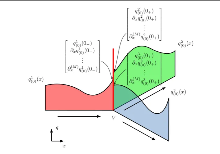
Figure 2.1:
Illustration of an initial condition for a J-GRP withN=3vessels and vertexV for a singlecomponent q(0)(x,t) of the vector of unknownsQ(0)(x,t). The dataq1
(0),q2(0) andq3(0) are smooth away from
vertexV and have one-sided spatial derivatives atV.
problem in terms of vessels. First, we define the J-GRP, then we explain how to solve the J-CRP for one-dimensional blood flow equations and propose a new solver for the J-GRP.
Consider a set of N vessels with the common vertexV. For thek-th vessel, variable xk is the local coordinate and the vertexV is located in 0 without loss of generality. In each k-th vessel, consider the following initial value problem
PDEs: ∂tQk+∂xF(Qk) =S(Qk), xk∈Ik= ak,bk
, t>0,
ICs: Qk(xk,0) =Qk(0)(xk),
)
(2.33)
where eitherak orbkis the local coordinate of vertexV, spatial domainI
khas lengthLk=|bk−ak|
and the initial conditionQk
(0)(xk)is a smooth vector-valued function of the local coordinatexk (e.g.
polynomials of orderM). Note that the material and geometrical properties can be different for each
k-th vessel. The set of solutionsQk(xk,t), with k=1, . . . ,N, has to satisfy the following coupling conditions at the common vertexV
φ(Q1(0,t), . . . ,QN(0,t)) =0, t>0, (2.34)
where the vectorφ defines coupling conditions. We define asJunction-Generalized Riemann
Prob-lem (J-GRP) at the vertexV withN vessels, the set initial value problems (2.33), withk=1. . . ,N,
2.2 Methods
17
We are interested in finding the solutions in time of problem (2.33) at the vertexV, which we denote withQk
V(τ), fork=1, . . . ,N, to evaluate the numerical fluxFkV of thek-th vessel at the vertex
V, namely
FVk = 1
∆t
Z tn+1
tn F(Q
k
V(τ))dτ. (2.35)
In the following we shall refer to these numerical fluxes at the vertexV as the junction-numerical
fluxes. The main ingredient we require to solve the J-GRP is the related classical version with
piece-wise constant data and no source terms.
The Junction-Classical Riemann Problem (J-CRP)
Consider the following set of initial value problemsPDEs: ∂tQk+∂xF(Qk) =0, x∈Ik= ak,bk
, t>0,
ICs: Qk(x,0) =Qk(0),
)
k=1, . . . ,N, (2.36)
with coupling conditionsφ
φ(Q1(0,t), . . . ,QN(0,t)) =0, t>0, (2.37)
whereQk
(0), withk=1, . . . ,N, are constant vectors. We define asJunction-Classical Riemann
Prob-lem (J-CRP)at the vertexV withN vessels, the set initial value problems (2.36), withk=1. . . ,N,
with constraints (2.37).
The solution of a J-CRP is a set of self-similar functions Dk(x/t)defined for each k-th vessel. For a 2×2 hyperbolic balance law system in subcritical regime, we have a total number of 2N
states. These 2N states arise from theN initial conditions Qk(0), with k=1, . . . ,N, and N states
Qk
∗, withk=1, . . . ,N, which are connected to the initial conditions through non-linear waves and
among themselves by the coupling conditions φ. To completely solve the J-CRP, one has to find
valuesQk∗, with k=1, . . . ,N, using both the structure of the waves (i.e. rarefactions or shocks) and the coupling conditionsφ. The solutions along thet-axisDk(0), withk=1, . . . ,N, of the J-CRP, are
termed here theGodunov states.
Here we present the solution of the J-CRP for the one-dimensional blood flow equations as-suming subcritical flow. To the authors’ knowledge, the complete solution of the J-CRP considering all possible wave-patterns is not available. This implies that we cannot handle supercritical and transcritical flows at junctions, which might be present in physiological situations due to vein col-lapse with discontinuous parameters in the human body, see [Siviglia 2013]. For the solution of the CRP for subcritical flows with discontinuous material properties for blood flow withn=0 and
m>0 refer to [Toro 2011], and to [Toro 2013] with n<0 and m>0. For arteries, [Han 2014] solved in complete detail the CRP with discontinuous material properties. For the solution of the J-CRP in blood flow for subcritical flows with n<0 and m>0, see also [Müller 2015a]. See
[Colombo 2008a, Colombo 2008b, Garavello 2006, Borsche 2014a] for the solution of the J-CRP
a1
0 =b1
a2= 0
a3= 0
b2
b3
Q1 (0)
Q2 (0)
Q3 (0) Q1
∗
Q2
∗
Q3
∗
f1
f2
f3
f4
f5
f6
t
x
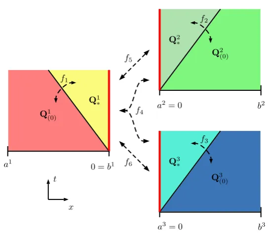
Figure 2.2:
Representation of a J-CRP for a typical2×2non-linear system with N=3 vessels, whereb1=0,a2=0anda3=0are the local coordinates of vertexV for the first, second and third vessel respectively.
The non-linear function fkconnects the initial conditionQk(0)and unknownQk∗fork=1. . . ,3, f4 connects all
the unknownsQ1
∗,Q2∗,Q3∗, while f5and f6 connect the unknownQ1∗toQ2∗ andQ3∗, respectively.
The coupling conditions that connect states Qk
∗, withk=1, . . . ,N, among themselves are
φ(Q1∗, . . . ,QN∗) =
N
∑
k=1
gkAk∗uk∗
pt(A1∗,u∗1;K1,A10)−pt(A2∗,u∗2;K2,A20) ..
.
pt(A1∗,u∗1;K1,A10)−pt(AN∗,u∗N;KN,AN0)
=0, (2.38)
where the vector of conserved variables Q is defined in (2.6), while Kk and Ak
0 are the material properties of thek-th vessel. The auxiliary functiongk indicates whether thek-th vessel has vertex
V at ak orbk, and reads
gk=
(
−1 ak=0,
1 bk=0, (2.39)
pt denotestotal pressure
pt(A,u;K,A0) =
1
2ρu
2+p(A;K,A
0), (2.40)
andpis the pressure given in (2.2). The first component ofφassures conservation of mass, whereas
2.2 Methods
19
(a)
(b)
Figure 2.3:
Example of a J-CRP. Piece-wise constant data are given for each vessel. Frames(a) and(b) depict the solution at initial and output time for a simple J-CRP respectively. A rarefaction wave propagates backward in the left sub-domain, whereas two shocks move forward in the others.components Ak∗ and qk∗=Ak∗uk∗, the total number of unknowns is 2N. This means that we need a total number of2N equations to close the system. The coupling conditionsφ containN equations, while the otherNequations are obtained by connecting each stateQk∗to the initial conditionQk(0)
through non-linear waves fork=1, . . . ,N. The total number of equations are2N and therefore the system is closed.
The non-linear relationship between Qk∗ andQk(0), withk=1, . . . ,N, reads
where the non-linear functionβ is
β(A∗;A,K,A0) =
Z A∗
A
c(τ;K,A0)
τ dτ ifA∗≤A, rarefaction wave,
r
B(A∗;A,K,A0)
A∗−A
A∗A ifA∗>A, shock wave.
(2.42)
The wave speed is
c(A;K,A0) =
v u u tK ρ m A A0 m −n A A0 n! , (2.43)
and the functionBis
B(A∗;A,K,A0) =
K
ρ
m
m+1
Am∗+1−Am+1 Am0 −
n n+1
An∗+1−An+1 An0
. (2.44)
Gathering the information coming from Eqs. (2.38) and (2.41) we end up with the following
Proposition 2.2.1. The solution of the J-CRP withNvessels for subcritical flow is found by solving the following non-linear system
f1(x1,y1;A1(0),u1(0)) =y1−u(10)+g1β(x1;A(10),K1,A10) =0,
.. .
fN(xN,yN;AN(0),uN(0)) =yN−u(N0)+gNβ(xN;A(N0),KN,AN0) =0,
fN+1(x1, . . . ,xN,y1, . . . ,yN) =g1x1y1+g2x2y2+···+gNxNyN =0,
fN+2(x1,y1,x2,y2) =pt(x1,y1;K1,A10)−pt(x2,y2;K2,A20) =0,
.. .
f2N(x1,y1,xN,yN) =pt(x1,y1;K1,A10)−pt(xN,yN;KN,AN0) =0,
(2.45)
where the unknowns of the problem are
X= [x1, . . . ,xN] = [A1∗, . . . ,AN∗], Y= [y1, . . . ,yN] = [u1∗, . . . ,uN∗], (2.46)
withβ and pt defined in(2.42)and (2.40), respectively.
The k-th non-linear function fk connects the initial condition Qk(0) to the unknown Qk∗ for
k=1, . . . ,N, fN+1 connects all the unknowns Q1∗. . . ,QN∗, and fk+N connects the unknown Q1∗ to
2.2 Methods
21
t
x ˆ
Q1
(0)(τ) Q1V(τ)
Q3
V(τ)
t= 0
t=τ
Q2
V(τ)
ˆ
Q3(0)(τ)
ˆ
Q2(0)(τ)
V
Figure 2.4:
Illustration of the MT-HEOC solver for the J-GRP with N=3vessels. The limiting values atvertexV are evolved separately up to timet=τ. The sought solutions along thet-axis are the Godunov states
of the J-CRP with these evolved states as initial data.
2.2.4
A new implicit J-GRP solver
Here we propose a new implicit solver for the J-GRP. Following the idea of the explicit HEOC solver for the J-GRP proposed in [Borsche 2016] and the implicit MT-HEOC solver for the GRP in
[Toro 2015a], we propose to combine them and construct the MT-HEOC solver for the J-GRP.
The J-GRP solutions along thet-axisQVk(τ), withk=1, . . . ,N, of (2.33) with coupling conditions
φ are found by solving the following J-CRP at the vertexV withN vessels and coupling conditions φ
PDEs: ∂tQk+∂xF(Qk) =0, x∈Ik= ak,bk
, t>0,
ICs: Qk(x,0) =Qˆk(0)(τ).
)
k=1, . . . ,N, (2.47)
where Qˆk
(0)(τ), with k=1, . . . ,N, are constant vectors. The evolved values Qˆk(0)(τ) are found by
applying for eachk-th vessel the implicit Taylor expansion at the vertexV up to timeτ, that is, by
solving the following non-linear problem: findUˆk(0) such that
L(Uˆk
(0);Uk(0),τ) =0, (2.48)
where the leading termUk
(0) is
Uk(0)= [Uk(,0
0), . . . ,U
k,M
(0)], U
k,j
(0)=
∂x(j)Qk(0)(0+) =xlim→0 +
∂x(j)Qk(0)(x), ifak=0, ∂x(j)Qk(0)(0−) = lim
x→0−∂
(j)
x Qk(0)(x), ifbk=0,
j=0, . . . ,M.
The solution procedure of the non-linear problems (2.48) is termed here theevolution stage. As in the MT-HEOC solver for the GRP, a possible initial guess for a numerical method to find solution of the non-linear problem (2.48) is Uk(0). Once we solve problem (2.48), then the evolved vector
ˆ
Qk
(0)(τ)will be the first entry ofUˆk(0), namelyUˆ
k,0
(0). The sought J-GRP solutions along thet-axis at
timet=τ are the Godunov states of the J-CRP (2.47) with initial data Qˆk(0)(τ), withk=1, . . . ,N, and self-similar solutionsDk(x/t), namely
QkV(τ) =Dk(0), k=1, . . . ,N. (2.50)
Assuming subcritical flow, the valuesQk
V(τ)are theNstatesQk∗described in Section2.2.3, namely
QkV(τ) =Q∗k, k=1, . . . ,N. (2.51)
We call the present method the MT-HEOC solver for the J-GRP, which extends the MT-HEOC solver for the GRP to the J-GRP. In the evolution stage of the MT-HEOC solver for the GRP, one applies an implicit Taylor series expansion to the left and right boundary extrapolated values, up to timet=τ; this part gives left and right evolved values that are the initial conditions for a CRP. The
solution along thet-axis of the GRP at timet=τis then the Godunov state of the CRP. The natural
generalization of the evolution stage of the MT-HEOC solver for the J-GRP is to apply an implicit Taylor series expansion on each vessel at the vertexV up to time t=τ; this part gives evolved
values that are the initial conditions for a J-CRP. The solutions along the t-axis of the J-GRP at timet=τ are then the Godunov states of a J-CRP.
See Figure2.4for an illustration of the MT-HEOC solver for the J-GRP where we haveN=3
vessels. We use