A New Sinusoidal Oscillator Circuit Using a Single Current Conveyor

(1)

Journal of Pure Applied and Industrial Physics Vol.1, Issue 3, 30 April, 2011, Pages (162-211)

A New Sinusoidal Oscillator Circuit Using a Single

Current Conveyor

NUTAN LATA

Department of Physics, Doranda College, Ranchi University, Ranchi-834 0082, India

ABSTRACT

A new sinusoidal oscillator circuit is presented using two capacitors, three resistors and a single current conveyor. The analytical expressions are obtained, both by assuming the current conveyor to be ideal and by taking the tracking errors into account. It has been shown that the slightly greater than unity value of loop gain required to maintain sustained oscillations is provided by taking the tracking errors into account. Simulation and experimental results are presented. The circuit presented generates perfectly sinusoidal waves in the audible frequency range and enjoys low sensitivity.

Keywords: CCII, Second generation current conveyor, Sinusoidal oscillator.

1. INTRODUCTION

The second generation current conveyor (CCII), introduced by Sedra and Smith1, is now widely used for implementing a number of high performance electronic functions. The use of current conveyor as the active element in the realization of transfer function was introduced by Soliman2. Since then, a number of circuits using current conveyor have been reported3-13. In this paper, a new sinusoidal oscillator circuit is presented using two capacitors, three resistors and a single current conveyor. It has been shown

that the slightly greater than unity value of loop gain required to maintain sustained oscillations is provided by taking the tracking errors into account. The circuit presented enjoys low sensitivity.

2. SECOND GENERATION CURRENT CONVEYOR (CCII)

(2)

Figure 1: Block diagram of second generation current conveyor

0

1

0

1 0

Y Y

X X

Z z

i

v

i

v









 









 

=









 











±



 





 

(1)

Thus, the terminal Y exhibits an infinite input impedance. The voltage at X follows that applied at Y, and thus, the terminal X exhibits a zero input impedance. The conveyor includes a positive sign if iX = iZ, that is, if both iX and iZ either enter into the conveyor or come out of the conveyor, and includes a negative sign if iX = - iZ, that is, if iX enters into the conveyor, iZ comes out of it and vice-versa.

3. CIRCUIT CONFIGURATION AND ANALYSIS

3.1 Assuming the current conveyor to be ideal

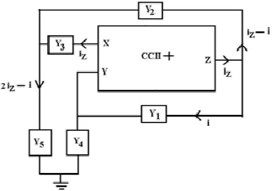
Consider the circuit shown in Figure 2. The distribution of currents is shown in this figure. For an ideal current conveyor, we have

,

0,

X Z Y X Y

i

=

i i

=

v

=

v

(2)

The potential at the terminal Z is

4 1 3

1 1 1

. ( ). (2 ).

Z Z Z

v i i i i i

Y Y Y

= = − + − (3)

Solving, it gives

4 3 1 1 3 3 4 1 4

(

2 )

.

_Z

Y Y

Y

i

Y Y



+



=





+





(4)

A direct analysis of the circuit shown in Figure 2 by taking vX = vY and using Equation (4) gives the characteristic equation as

Figure 2: Block diagram of proposed sinusoidal oscillator circuit showing the current distribution, assuming the current conveyor to be ideal

3

(

1 4 2

)

4

(

1 2

)

0

Y Y

+ −

Y

+

Y Y

+

Y

=

(5)

Let

where s= j

ω

and

G

=

1/

R

. Equation (5) then gives

- (6)

Equating imaginary parts on both sides of Equation (6), we get

1 3 4

2 3

C C

R

R C

+

= (7) 1 1, 3 3, 2 2, 4 4

Y =sC Y =sC Y =G and Y =G

2

1 3 [ 1 4 3( 4 2)] 2 4

C C j C G C G G G G

(3)

as the condition of oscillation. Equating real parts on both sides of Equation (6) and using the condition of oscillation as given by Equation (6), we get

2 4 0

1 3 2 4 1 3

1

G G

C C

R R C C

ω

=

(8)

as the frequency of oscillation. The corresponding circuit is shown in Figure 3.

3.2 When the tracking errors are taken into account

When the tracking errors are taken into account, the voltage and current relationships between input and output become

(1

) ,

(1

)

X v Y Z i X

v

= −

ε

v i

= −

ε

i

(9)

The distribution of currents in this case is shown in Figure 3. The potential at the terminal Z is

4 1 3

1 1 1

. ( ). ( ).

Z Z Z X

v i i i i i i

Y Y Y

= = − + + − (10)

Solving the above equation, we get

4 3 1

1 3 3 4 1 4

[(1 ) (2 ) ] .

i i

X

Y Y Y

i i

Y Y Y Y Y Y

ε

− + −

=

+ + (11)

Again, taking

v

_X

= −

(1

ε

_v

) ,

v

_Y we get, on simplification, the characteristic equation as

3 1 4 2

1 4 1 2 2 4

[ (1 )(1 )]

(2 ) 0

i v

Y Y Y Y

Y Y Y Y Y Y

ε

ε ε

+ − − − +

+ − + = (12)

When

Y

1

=

sC Y

1

,

3

=

sC Y

3

,

2

=

G

2

,

and 4 4

,

Y

=

G

Equation (12) gives

2

1 3 3 4 2

1 4 1 2 2 4

[

{

(1

)(1

)}

(2

)

]

i v

C C

j

C G

G

C G

G G

ω

ε

ε ε

−

+

−

+

+ −

= −

(13) Equating imaginary parts on both sides of

Equation (13), we get

3 4 2 1 4 2

[

(1

)(1

)

[

(2

)]

0

i v

v i

C G

G

C G

G

ε

−

+

−

=

(14)

Figure 3: Block diagram of proposed sinusoidal oscillator circuit showing the current distribution, when the tracking errors are taken into account

Solving, Equation (14) gives

1 3 4

2 (1 i)(1 v) 3 (2 i) v 1

C C

R

ε

C

ε ε

C

+ =

− − − − (15)

as the condition of oscillation.

Equating real parts on both sides of Equation (14) and using Equation (15), we get

0

2 4 1 3

1

R R C C

(4)

Journal of Pure Applied and Industrial Physics Vol.1, Issue

as the frequency of oscillation.

It is easy to see that the conditio oscillation as given by Equation (15) reduces to that given by Equation (7) for an ideal current conveyor when the tracking errors are neglected. A detailed calculation, by taking

ε ε

_i

= =

_v

0.03,

shows that the ratio

4

/

2

R

as demanded by Equation (15) for the circuit shown in Figure 2 to oscillate is about 6.8% higher than that demanded by Equation (7). This theoretical result has actually been verified experimentally.

4.

ω

0

−

SENSITIVITY

The various sensitivity figures are calculated using the sensitivity definition

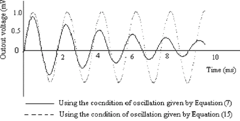
Figure 4: Computer simulation of the circuit shown in Figure 2 with the condition of oscillation given by Equations (7) and (15)

Journal of Pure Applied and Industrial Physics Vol.1, Issue 3, 30 April, 2011, Pages

(162-as the frequency of oscillation.

It is easy to see that the condition of oscillation as given by Equation (15) reduces to that given by Equation (7) for an ideal current conveyor when the tracking errors are neglected. A detailed calculation, by shows that the ratio as demanded by Equation (15) for the circuit shown in Figure 2 to oscillate is about 6.8% higher than that demanded by Equation (7). This theoretical result has actually been verified experimentally.

The various sensitivity figures are calculated using the sensitivity definition

0 0

0

.

x

x S

x

ω

∂ =

∂

where x is the element of variation. Using Equation (17), the

ω

0

−

sensitivity for the circuit shown in Figure 2 was calculated and in each case, it was found to be –

5. SIMULATION RESULT

A computer simulation of the circuit shown in Figure 2 is shown in Figure 4 using the condition of oscillation as given by Equation (7) and by taking C1 =

R2 = 1 k, R4 =2 k. and C3 = 0.3µ

that the oscillations eventually die out. But, when this circuit is simulated by using the condition of oscillation as given by Equation (15) and by taking C1 = C3 = 0.1

k, and R4 =2.135 k, the circuit produces a pure sinusoidal wave.

Computer simulation of the circuit shown in Figure 2 with the condition of oscillation given by

-211)

(17) is the element of variation. Using sensitivity for the circuit shown in Figure 2 was calculated and

–1/2.

A computer simulation of the circuit shown in Figure 2 is shown in Figure 4 using the condition of oscillation as given by = C3 = 0.1µF,

µF. It is seen that the oscillations eventually die out. But, when this circuit is simulated by using the condition of oscillation as given by Equation = 0.1µF, R2 = 1 =2.135 k, the circuit produces a

(5)

Journal of Pure Applied and Industrial Physics Vol.1, Issue 6. EXPERIMENTAL RESULT

The circuit shown in Figure 2 has been experimentally studied using AD844 in the laboratory using various values of circuit components that satisfy the condition of oscillation as given by Equation (16). The components used were accurate to

The circuit is found to produce good, highly stable sinusoidal oscillations in the audible frequency range. The experimental data obtained by taking C1 = C3 = 0.1

k, and R4 =2.135 k is plotted in Figure 5 together with the simulated data to facilitate comparison. From Figure 5, it may be seen that the experimental data are in close

Figure 5: Simulated and experimental curves for the circuit shown in Figure 2 using the condition of oscillation given by Equation (15)

It has been shown that the slightly greater than unity value of loop gain required to maintain sustained oscillation is provided by taking tracking errors into account.

Journal of Pure Applied and Industrial Physics Vol.1, Issue 3, 30 April, 2011, Pages (162-6. EXPERIMENTAL RESULT

The circuit shown in Figure 2 has been experimentally studied using AD844 in the laboratory using various values of circuit components that satisfy the condition of oscillation as given by Equation (16). The components used were accurate to ± 5%. it is found to produce good, highly stable sinusoidal oscillations in the audible frequency range. The experimental data = 0.1µF, R2 = 1 =2.135 k is plotted in Figure 5 together with the simulated data to facilitate comparison. From Figure 5, it may be seen that the experimental data are in close

agreement with the simulated curve. The minor deviation of the experimental curve from the simulated curve may be attributed to the mismatching of the component values used in the experiment.

7. CONCLUSIONS

A new current conveyor based sinusoidal oscillator circuit is presented. The circuit presented exhibits the following salient features:

1. It uses a single current conveyor. 2. It has low sensitivity characteristics. 3. Adjustment is easy.

Simulated and experimental curves for the circuit shown in Figure 2 using the condition of oscillation given by Equation (15)

that the slightly greater than unity value of loop gain required to maintain sustained oscillation is provided by taking tracking errors into

REFERENCES

1. Sedra & Smith, IEEE Trans. Circuits & Systems, 17, 132 (1970).

2. Soliman A M, Int. J. electroni (1975).

-211)

agreement with the simulated curve. The minor deviation of the experimental curve from the simulated curve may be attributed to the mismatching of the component values

A new current conveyor based sinusoidal oscillator circuit is presented. The circuit presented exhibits the following

It uses a single current conveyor. It has low sensitivity characteristics.

Simulated and experimental curves for the circuit shown in Figure 2 using the condition of

(6)

3. Chong C P & Smith K C, Int. J. Electronics, 62, 515 (1987).

4. Abuelma’atti M T , & Al-Qautani M A, IEEE Trans. Circuits and Systems II: Analog and Digital Signal processing, 45, 881 (1998).

5. Martinez P A, Sabaddi J, Aldea C & Celma S, IEEE Trans. Circuits and systems I: Fundamental Theory and Applications, 46, 1386 (1999)

6. Horng J W, Int. J Electronics, 88, 659 (2001).

7. Barthelemy H, Meillere S and Kussener E, Electronics Letters, 38,1254 (2002). 8. Khan A A, Bimal S, Dey K K and Roy S

S, IEEE Trans. Instrumentation and

Measurements, 54, 2402 (2005).

9. Bhaskar D R and Senani R, IEEE Trans. Instrumentation and Measure-ments, 55, 2014 (2006)

10. Kumar P, Pal K & Gupta G K, Indian J Pure & Applied Physics, 44, 398 (2006). 11. Chung-Ming Chang, Soliman A M & Swamy M N S, IEEE Trans. On Circuits & Systems, 54, 1430 (2007).