Consistency of the Douglas – Rachford Splitting Algorithm for the Sum of Three Nonlinear Operators: Application to the Stefan Problem in Permafrost Soils

(1)

Published online August 10, 2013 (http://www.sciencepublishinggroup.com/j/acm) doi: 10.11648/j.acm.20130204.11

Consistency of the Douglas – Rachford splitting algorithm

for the sum of three nonlinear operators: application to

the Stefan problem in permafrost soils

Taras A. Dauzhenka

*

, Igor A. Gishkeluk

R&D Dept., Simmakers Ltd., 1A-307 V. Kharuzhei str., 220005 Minsk, Belarus

Email address:

[email protected](T. Dauzhenka)

To cite this article:

Taras A. Dauzhenka, Igor A. Gishkeluk. Consistency of the Douglas – Rachford Splitting Algorithm for the Sum of Three Nonlinear Operators: Application to the Stefan Problem in Permafrost Soils. Applied and Computational Mathematics.

Vol. 2, No. 4, 2013, pp. 100-108. doi:10.11648/j.acm.20130204.11

Abstract:

Consistency of the Douglas – Rachford dimensional splitting scheme is proved for the sum of three nonlinear operators constituting an evolution equation. It is shown that the operators must be densely defined, maximal monotone and single valued on a real Hilbert space in order to satisfy conditions, under which the splitting algorithm can be applied. Numerical experiment conducted for a three-dimensional Stefan problem in permafrost soils suggests that the Douglas – Rachford scheme produces reasonable results, although the convergence rate remains unestablished.

Keywords:

Splitting Algorithms, Alternating Directions Scheme, Stefan Problem, Nonlinear Heat Equation, Consistent Approximation

1. Introduction

Formulation of the splitting and alternating directions implicit methods (ADI methods) in late 1950-s – early 1960-s [1 - 9] was followed by its rapid developments [10 - 14] and applications in various fields ranging from partial differential equations (PDE) [15, 16] to complex optimization problems [17 – 19]. The reason for such a wide application of these methods is related with a possibility to capture different aspects of a studied system, which are reflected in a complicated PDE, solved by the splitting methods. The complexity of a particular PDE may be due to the presence of terms (operators) that are mathematically very different, making this PDE hard to analyze. In this case, splitting methods provide one with a possibility to split the equation into a set of sub-equations, where each sub-equation is of a type, for which simple and efficient methods are available. The main two ideas for splitting of PDEs are the following (see, e.g. [20]):

1. Physical splitting (related to the underlying processes).

2. Mathematical splitting (related to abstract matrices, found in the differential equations after spatial discretization).

The overall numerical method is then formed by

choosing an appropriate numerical scheme for each sub-equation of the initial PDE and combining the schemes together by operator splitting [21].

Following the classification proposed by Marchuk [11], the factorization and ADI methods, based on inhomogeneous approximation of auxiliary (intermediate) steps, will be called the splitting methods. Under an inhomogeneous finite difference scheme we imply a scheme, for which the coordinate shifts do not induce grid functions from the space, on which the difference operators of the scheme are defined (more details and formal notion of such schemes are developed in [22]). Thus, each intermediate step not necessarily approximates the original problem, but in the whole the approximation takes place. Indeed, the Douglas - Rachford splitting algorithm [6, 23], the study of which is presented in this paper, comprises three steps, each of which separately does not approximate the original problem:

1 1 1

1 1 1 (1)

or, the same, 1 step:

1 1 1

(2)

2 step:

1 1

1 1 1

(3)

3 step:

1 1 1

(4)

where is the iteration parameter, _{, ,} are some operators and n is the iteration index. From (2) - (4) one can see that the intermediate quantities and do not belong to the space of functions that approximate solution of the original problem, while and are the consecutive iterations of . To conclude this discussion of relation between ADI and splitting methods we note that in [24, 19] it was shown that the Douglas – Rachford splitting method for minimization of the sum of two monotone operators is a special case of proximal point algorithm.

It is known that the algorithm (1) is absolutely stable if the operators _{, ,} are linear [6, 23]. There has been made numerous attempts to generalize the Douglas - Rachford, Peaceman - Rachford and other splitting algorithms to the case of nonlinear problems [25 – 31]: in [31] a solution-set characterization is used for the estimation of convergence rate of Douglas – Rachford algorithm, applied to variational inequalities and minimization problem with the sum of two convex functions; in [27] the operator-theoretical approach is employed for the studies of convergence of Lie and Peaceman – Rachford splitting, applied to quasilinear parabolic problems with the sum of two nonlinear operators; in [32] the weak convergence of the Douglas – Rachford algorithm was proved for the minimization problem with the sum of two general maximal monotone operators in infinite dimensional spaces; in [33] weak convergence has been proved for an abstract family of projective splitting algorithms for sums of arbitrary numbers of maximal monotone operators (Propositions 3.2 and 4.2 in [33]), but no convergence rate has been established. It has also been demonstrated that the problem with the analysis of dimensional splitting algorithms for the solution of nonlinear differential equations (or equations with variable coefficients) is due to non-commutativity of operators [25]. Despite all these attempts, to the best of our knowledge there is no complete convergence analysis and convergence rate estimation for the problems, comprising the sum of three nonlinear operators available in the literature.

In this paper we present the study of consistency of the algorithm (1) (in application to evolution equations) for the

case when operators _{, ,} are non-linear. For this purpose we employ the results published in [17, 34, 35] and make some additional assumptions that are natural from the point of view of application of the algorithm (1) to Stefan problem in permafrost soils.

The paper is organized as follows: next section contains the theoretical framework and the list of assumptions; in Section 3 the proof of consistency for the algorithm (1) in application to evolution equations is presented; Section 4 is dedicated to the application of algorithm (1) to Stefan problem in permafrost soils. Section 5 presents some numerical results and is followed by conclusions.

2. Notation and Setup

2.1. Theoretical Framework for the Consistency Studies

Let us consider an evolution equation of the form:

/ 0, (5)

0 , 0 ∞

where H is a Hilbert space and : ! .

From the theory of nonexpansive semigroups it is known that [36, 37 Corollary 31.1]

Proposition 2.1: If the operator A is maximal accretive and is the unique solution of Eq.(5), then

" (6)

where # and " is a nonlinear nonexpansive semigroup on , which can be uniquely extended to a nonexpansive semigroup on . The generator of

" on is $ .

Let us remind that the maximal accretive operator is defined as follows:

Definition 2.1: Let : ! be an operator on the real Hilbert space H. Operator A is called maximal accretive if and only if:

For any % & 0: ' % : ! is injective and

' % is nonexpansive on H.

In our analysis we will make use of the following result [38]:

Proposition 2.2: Let : ! be an operator on the real Hilbert space H. Then the following two properties of operator A are equivalent:

(i) A is maximal accretive (ii) A is maximal monotone

The maximal monotone operator is defined as follows: Definition 2.2: Let : ! be an operator on the real Hilbert space H provided with an inner product , . Operator A is called maximal monotone if and only if the following two conditions hold:

(i) $ (, $ ( ) 0 for any , ( #

(ii) If * $ (, $ ( ) 0 for any ( # ,

then *.

(3)

our further analysis of consistency [34 Corollary 4.3, 35 Theorem 4.3]:

Theorem 2.1: Let : ! be a maximal accretive densely defined operator and let " be a semigroup generated by $ . Let + , be a family of contractions with the Lipschitz constant - , defined on a closed convex subset . for all , & 0. If

(i) - , 1 / , for , ! 0 (7)

(ii) lim_3! ' 4₃ ' $ + , 5 ' 5

(8)

for 65 # 7 . and 6 & 0.

Then, for 65 # 7 ., the following result holds:

lim ! 8+ /9 ! " (9)

And the limit is uniform on bounded intervals of

# :0, ∞ .

Proof of this theorem can be found in [34, 35].

Another important result that we will employ in our study is the following Lemma proved in [17]:

Lemma 2.1: Let : ! be a maximal monotone operator. If for every # and ₄# there exists a limit

lim4! 4$ / ;, (10)

Then

lim4! <= > 4? @A

4 B?< ; (11)

where B_?< ; denotes the projection operator for vector y

onto the range of A.

The results presented above constitute the basis for the application of nonlinear semigroup theory to the consistency analysis of splitting schemes. In the next Subsection we will make some additional assumptions that are necessary for the specific case of dimensional splitting in the Douglas – Rachford scheme and in Section 3 we will use the Theorem 2.1 and Lemma 2.1 in order to study consistency of this algorithm.

2.2. Finite Differences Formalism for the Quasilinear Heat Equation

The equation describing heat transfer in a system with phase transition has the following form:

. C<_CD EF( G HIJE (12)

where 5, ;, K, is the unknown function (temperature: _L # M NO at every fixed _L, M NO being a real linear space of positive valued functions),

. is the heat capacity, G is thermal conductivity. By Ω we denote a bounded, open subset of an Euclidian space Q with boundary ΩR, the closure of Ω being

denoted by NO.

Following the classification given in [39], we call (12) a quasilinear heat equation. The initial and boundary conditions are taken to be:

5, ;, K, 0 S 5, ;, K, | 5, ;, K # Ω (13)

5, ;, K, S 5, ;, K, | 5, ;, K # ΩR, # U (14) We consider the cases when . ) % & 0 and

G ) V & 0, thus (12) is uniformly parabolic and has a unique solution to the initial-boundary-value problem (13)--(14) [40].

For the formulation of finite difference scheme we introduce the following discretization procedure. Let the vector W W_X, W_Y, W_Z # Q have positive coordinates and [_\ be the set of all points F ] W_X, ^ ] W_Y, G ] W_Z # Q , the indices F, ^, G being integers. Two points 5 F ]

WX, ^ ] WY, G ] WZ and 5 F ] W_X, ^ ] W_Y, G ] W_Z belonging to [_\ are called neighbors if

_ F $ F ] WX ^ $ ^ ] WY G $ G ] WZ

WX,Y,Z. The points 5 # [_\7 Ω, all of whose neighbors belong to Ω`, are denoted by Ω_\.

Following [41], we denote the points 5 # [_\\Ω_\ with the property that at least one neighbor belongs to Ω_\ by

ΩR\. Thus, the full spatial mesh is Ω`_\ Ω_\b ΩR_\, ΩR_\ being the set of boundary points (outside of Ω_\). For the following we assume that Ω`_\ is a homogeneous (i.e.,

WX, WY, WZ are constants) cubic domain.

Let d :0, ∞ and d d\ 0. Then the time mesh is defined as follows:

de # d, f ] g, 9 0,1, … (15)

The approximate solutions of (12), , are defined on

de and take their values in a real finite-dimensional linear

space M Ω`_\ , the dimension of which is equal to the number of points in Ω`_\. A function # M Ω`_\ is called admissible if 0 S 5, ;, K and

5, ;, K, on ΩR_\i d_e. As was pointed out in [41],

5, ;, K, is, in general, not known in ΩR_\i d_e and thus the following assumption should be made: there exists a null sequence (that converges to zero) W_X,Y,Zj of mesh spacings such that Ω_\kl Ω and W_X,Y,Z always belongs to the sequence W_X,Y,Zj . This assumption guarantees that an admissible function is uniquely specified in [_\i

de \ Ω\i de in terms of the initial and boundary values

of 5, ;, K, .

For every # M Ω`_\ we define the first-order forward and backward difference operators:

mWn] n o $ o

Wn] n o $ o

p

(16)

where q 5, ;, K , 2 s F_ns EFf_n Ω`_\ $ 1 ,

(4)

G_ot / , G uvotA uvo (17)

Thus, G_o_{t / ,} are the values of G at the

fictitious intermediate nodes of the mesh Ω_\ at g ]

9 # de, # M Ω`\ .

From the Eqs. (16)--(17) one obtains:

$ _owG ] _o x _\

vo(Λo, +Λo, )U, (18)

where

zΛo, Go / , ]

u_vo@A u_vo \_vo Λ_o, Go / , ]

u_vo{A u_vo \_vo

p (19)

and G corresponds the value of G at

g ] 9 # de, # M Ω`_\ , F_n and q being defined as

q 5, ;, K ; 1 s F_ns EFf_n Ω`_\ .

We also provide M Ω`_\ with the | -inner product

, } and induced norm ~ ~ , / on Ω`_\:

, } WX] WY] WZ∑•#‚ƒ € } € (20)

The maximum norm is defined as following:

~ ~8 max (21)

We define on Ω`_\ a modified A-inner product , } _,? and induced norm

~ ~ ,? , /,?

by

, } ,? WX] WY] WZ∑n X,Y,Z ∑•#‚ƒ € ,n} €

(22)

,nw} € x $. } € ] n G } € n} €

(23)

where . } € and G } € correspond the values of . ( 5, ;, K, and G ( 5, ;, K, at €

5, ;, K # [\, g ] 9 # de , ( # M Ω` respectively.

Note that the so defined operator _,n implies that it is generally not true that _,n: M Ω`_\ ! M Ω`_\ .

Now we can write the following Douglas – Rachford finite differences scheme for the heat equation (see detailed discussion of this scheme in [42]):

w1 g ] ,Xxw1 g ] ,Yxw1 g ] ,Zx e

∑n ,n (24)

where _,n are given by (23), q 5, ;, K , _e

$ /g, and g at

9 ] g # de, # M Ω`_\ .

Application of the scheme (24) to the Stefan problem will be studied in Section 4.

To complete this Section we present the following two

assumptions that are necessary to guarantee computational stability of this scheme [42]

Assumption 2.1: In the scheme (24) the operators _,n are acting on the vectors in the following way:

,n $. ] n G n (25)

This assumption leads to consideration of a linear finite-difference scheme of type (24) for the heat equation with variable coefficients . and G , the forms of which depend on the temperature field calculated at the previous time level. This kind of assumption is commonly used when considering nonlinear time dependent problems (e.g., [26]).

Let us rewrite (25) in the following equivalent form:

,nw} € x † ,nw} € x ‡ ,n } € (26)

where

z † ,nw} € x

ˆ_vo,‰{ Šo{Šo@‹ • Œ‰

‡ ,nw} € x ˆvo,‰

@ _Š_o{ _Š_o@_{‹ •} Œ‰

p

, (27)

• Žo, Go A•, Go A•, /2

Ž_o, G_o A

•, $ Go A•, / 2 ] Wn

p

. (28)

Assumption 2.2: The functions . : M Ω`_\ ! ℓ8 Ω`_\ ,

Ž : M Ω`\ ! ℓ8 Ω`\ and Ž : M Ω`_\ ! ℓ8 Ω`_\ (defined by (17) and (28)) are mapping the elements € #

M Ω`\ into a sequence space ℓ8 Ω`_\ , the elements of which ( Ž € , Ž € , . € # ℓ8 Ω`_\ ) satisfy the following relations:

‘| n. w. € | s ’ ] . €€ x . €

| n . € | s ’ ] . €

p

(29)

“ ”

•Ž w € x Ž € –vo{A•,‰• –vo@A•,‰•

| n Ž € | s ’ ] Ž €

p

(30)

“ ”

•Ž w € x Ž € –vo{A•,‰• –vo@A•,‰•

| n Ž € | s ’ ] Ž €

p

(31)

where the operators _n, _n are defined similarly to (16);

’ , ’ , ’ are real positive constants. ℓ8 Ω`_\ is the Banach space with the maximum norm.

3. Consistency of the

Douglas – Rachford Splitting Scheme

(5)

(32)

we have to make the following assumptions. Assumption 3.1: The operators

, , : , , ! (33)

and

are single valued, densely defined and maximal monotone on a Hilbert space H.

Assumption 3.2: The range of ' $ is dense in H for all & 0.

These two assumptions lead to the following important result:

Lemma 3.1: If Assumptions 3.1 and 3.2 are valid, then

HIJ€W

OOOOOOOOOOOOOOOOOOOOOOOOOOOO HIJ€W

The proof of this Lemma is presented in [27].

Now we are ready for the formulation of the main Theorem of consistency analysis for the Douglas – Rachford scheme.

Theorem 3.1: Let the Assumption 3.1 and Assumption 3.2 hold. Then, the family of contractions

+ —?4˜—?4•—?4Aw x ' (34)

defined on a closed convex subset . for all

& 0 with

—?4v™ A,•,˜ ' , , , (35)

satisfies the conditions (i) and (ii) of the Theorem 2.1 and

– $ generates a semigroup " such that " and

lim_{! 8}+ /9 ! "

holds for the evolution equation (5).

Proof: Satisfaction of the first condition of the Theorem 2.1 is obvious when taking the limit lim_4! + .

For the proof of satisfaction of the second condition of the Theorem 2.1 let us consider the following quantity:

1

4$ + 4 1 —?4˜—?4•—?4A w—?4Ax w—?4•x

w—?4˜x $ 3 4 (36)

Note that in general case when the operators _{, ,}

are nonlinear, —_?4_v, —_?4_v and —_?4_œ do not commute with

each other. At the same time, if _{, ,} are single valued,

one has the following identity:

w' , , x—?4_{v™ A,•,˜} ' (37)

Thus, we have for (36):

1

4$ + 4 1 —?4˜—?4• —?4˜—?4A —?4•—?4A

$3—?4˜—?4•—?4A —?4˜—?4••—?4A, w—?4•x ž

—?4˜•—?4•, w—?4˜x ž —?4A —?4˜—?4•:—?4A, w—?4˜x Ÿ 4 (38)

where

—?4v, ¡—?4œ¢ t

£ —?4v —?4 tœ $ —?4 tœ —?4v (39)

Proceeding in the same manner we obtain the following expression:

1

4$ + 4 1 —?4•—?4Aw 4$ —?4˜ 4x

—?4˜—?4Aw 4$ —?4• 4x

—?4˜—?4•w 4$ —?4A 4x

—?4˜¤—?4A, —?4•¥ 4 —?4˜—?4••—?4A, w—?4•x ž 4

—?4˜•—?4•, w—?4˜x ž —?4A 4

—?4˜—?4••—?4A, w—?4˜x ž 4

—?4•¤—?4A, —?4˜¥ 4 :—?4•, —?4˜Ÿ—?4A 4. (40)

Taking the limit at ! 0 and applying Lemma 2.1 under the condition

lim_{!8 4 D/}

we obtain:

lim_{4! 4 4}$ + 4 B?A< 0 B?•< 0 B?˜< 0 (41)

Thus, the operators (34) satisfy the conditions (i) and (ii) of the Theorem 2.1. Assumption 3.1 and Assumption 3.2 together with the Proposition 2.2 lead to the conclusion that operators

, , : , , !

and are maximal accretive. Finally, Proposition 2.1 leads to the conclusion that $ $

generates a semigroup " such that

" and

lim_{! 8}+ /9 ! "

(6)

completed.

Corollary 3.1: The algorithm (1) provides a consistent approximation for the evolution equation (5).

Proof: The statement becomes obvious when the algorithm (1) is put in the form:

+ .

4. Application to Stefan Problem in

Permafrost Soils

4.1. Stefan problem in permafrost soils

Following [42], we introduce some additional notations and notions that are necessary for the study of Stefan problem in permafrost soils.

Basing on results of [43 - 45], we formulate the model for the Stefan problem without explicitly invoking the front-tracking condition. This approach is justified by the observations that in case of explicit front-tracking models applied to Stefan problem in salted permafrost soils, there appears an overcooled region (frozen fringe zone) [46, 47] (the analysis of this zone and related frost heave and cryogenic suction processes [48, 49] are beyond the scope of the present work). Thus, we take into account the phase transition by introducing effective heat capacity ._¦LL , which incorporates the latent heat per unit mass § :

•.¦LL . $ 1 $ ¨ ] ©ª] § «ª <«<

. .D\ .L$ .D\ ] ¨

p

, (42)

¨ •1 $ ¬] -®ƒ < , s d•\

0, & d•\

p

(43)

where ._D\ and ._L are the values of volumetric heat capacities of the soil in thawed and frozen phases respectively, ¨ is the fraction of frozen water, " is the smoothing parameter, d_•\ is the phase transition temperature, ©_ª is the density of water. The thermal conductivity is taken to be

G GD\ GL$ GD\ ] ¨ (44)

where G_D\ and G_L are the values of thermal conductivities in thawed and frozen phases respectively.

4.2. Consistent Approximation for the Quasilinear Heat Equation

In Section 3 we have shown that the algorithm (1) can be used for a consistent approximation of evolution equation comprising the sum of three nonlinear operators. Let us now show that the scheme (24) provides a consistent approximation for the quasilinear heat equation (12).

Proposition 4.1: Let the Assumption 2.1 hold and let

. } € and G } € correspond the values of

. ( 5, ;, K, and G ( 5, ;, K, at € 5, ;, K #

[\ , g ] 9 # d_e , ( # M Ω` respectively. If

. ( .¦LL ( (in accordance with (42) - (43)) and

G ( is defined by (43) - (44), then the scheme (24):

w1 g ,Xxw1 g ,Yxw1 g ,Zx e ¯ ,n

n

gives a consistent approximation for equation (12):

. C<_CD EF( G HIJE .

Proof: The scheme (24) takes the form of the algorithm

(1) if we put g and _, _X,Y,Z _, _{, ,} .

According to the Theorem 3.1 and Corollary 3.1, algorithm

(1) provides a consistent approximation for the evolution

equation of type (5) if all the operators

F 1,2,3: F 1,2,3 !

and

are

(i) densely defined, (ii) single valued,

(iii) maximal monotone on a Hilbert space H. The first property comes from the definition of linear space M Ω_\ , given in Subsection 2.2. Indeed,

w , , x M Ω\ and M Ω\ .

The second and third properties come from the definition of . } € , G } € and from the fact that all the components of an admissible function # M Ω_\ are positive (see Subsection 2.2).

Thus, the scheme (24) satisfies the consistency property (9). Proof is completed.

In [42] the sufficient criterion for the computational stability of the algorithm (1) has been obtained. Below we present without proof the formulation of the main theorem for the analysis of computational stability of algorithm (1) (the proof can be found in [42]):

Theorem 4.1: Let the operators _,n (defined by (25)) satisfy the following condition for any 9 # d_e

1 $ ’°]

± ∑n ,n s ∑n ,ns 1 ’°] ± ∑n ,n,

(45)

where ± ~ $ ~₈, ’_°& 0 is a constant. Then the relation:

w1 g ,Xxw1 g ,Yxw1 g ,Zx ) e_²∑n ,n, (46)

(7)

where , # M Ω`_\ are the solutions of Eq.(24). Application of this theorem to the scheme (24) leads to the following stability criterion [42]:

e \o• s

² ²

³´µ ˆ‰{ ³¶· Œ‰

³´µ Œ‰

³¶· ˆ‰{ ] ’ , (48)

where ’ is a constant. The criterion (48) is sufficient for relation (47) to hold, which reflects the notion of computational stability.

Thus, for the linearized finite differences scheme (24) we have proved the consistency and the stability criterion is obtained in [42]. With these results we can proceed further and analyze the numerical experiments.

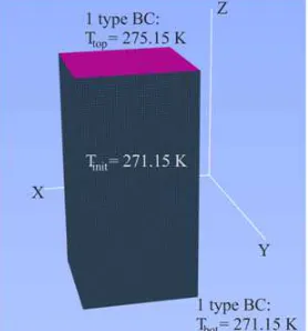
Figure 1. Rectangular parallelepiped with the mesh used in numerical experiment.

5. Numerical Experiment

Let us consider a rectangular parallelepiped with dimensions

5:fŸ i 5:fŸ i 10:fŸ

and following initial and boundary conditions (see Fig. 1):

dD¹• 275.15:ŽŸ d¼¹DD¹½ 271.15 :ŽŸ

d D 271.15 :ŽŸ

On the side edges of this parallelepiped zero thermal fluxes are posed.

Let us suppose that the specific heat and thermal conductivity of material in this parallelepiped are given by (42) – (44) with the following values of constants:

.D\ 1.89 :-—/ f Ž Ÿ,

.L 1.74 :-—/ f Ž Ÿ,

GD\ 0.7 :Á/ fŽ Ÿ,

GL 0.75 :Á/ fŽ Ÿ, d•\ 273.15 :ŽŸ,

" 10:Ž Ÿ,

§ 334 :G—/GHŸ,

Let us employ a homogeneous mesh with Δ5 Δy

Δz 0.1 :mŸ and the following number of nodes:

51 i 51 i 100. Using stability criterion (48) we obtain the values g 1160 :ÆŸ for the maximal time step and 744 for the minimal number of iterations.

In Fig. 2 the calculation results are presented for the time period of 10 days. Every contour plot in Fig. 2 presents a temperature field in the plane of parallelepiped with the coordinate x = 7 [m].

Figure 2. Contour plots of the temperature field at the planes x = 7 [m] obtained with the scheme (24) at different time moments.

One can observe a slight shift of the freezing front into the depth of soil. In order to demonstrate the change better, we plot the dependence of temperature on the coordinate in Fig. 3.

In Fig. 3 the same results as in Fig. 2 are presented in the form of temperature change with the depth along the line with coordinates x = 7 [m], y = 13.6 [m].

One can observe the phase transition point and different behavior of temperature field below and above that point. This is in agreement with Eq. (42) – (44) and the general expectations for the results of solution of a Stefan problem.

(8)

6. Conclusions

We have shown that the Douglas – Rachford splitting algorithm (1) can be employed for a consistent approximation of evolution equation of type (5) (Theorem 3.1 and Corollary 3.1), provided the operators

, , : , , !

and

are single valued, densely defined and maximal monotone in a Hilbert space H.

We suggest that the finite differences scheme (24) gives a consistent approximation for the heat equation (12) and can be used for the study of Stefan problems (Proposition 4.1). The conducted numerical experiment (with the computational stability criterion taken from [42]) provides evidence that the Douglas – Rachford dimensional splitting algorithm can be used for the studies of heat transfer in permafrost soils (we argue that all other experiments (with different parameters) were also successful). Although the numerical experiments conducted with the stability criterion (48) appear to be successful, we note that the convergence rate has not yet been established for the scheme (24) and this presents an open problem.

References

[1] N. N. Yanenko, The method of fractional steps: The solution of problems of mathematical physics in several variables, 1st ed. Springer- Verlag, (1971).

[2] Ye.G. D'yakonov “On the application of disintegrating difference operators”, USSR Computational Mathematics and Mathematical Physics, vol. 3, no.2, (1963), pp. 511 – 515.

[3] A.A. Samarskii “On the convergence of the fractional step method for heat conductivity equation”, USSR Computational Mathematics and Mathematical Physics, vol. 2, no.6, (1963). Pp. 1347 – 1354.

[4] A.A. Samarskii “Local one dimensional difference schemes on non-uniform nets”. USSR Computational Mathematics and Mathematical Physics, vol. 3, no. 3, (1963), pp. 572 – 619.

[5] G. I. Marchuk “On the theory of the splitting-up method”. Proceedings of the 2nd Symposium on Numerical Solution of Partial Differential Equations (1970), SVNPADE, pp. 469 – 500.

[6] J. Douglas, “Alternating direction methods for three space variables,” Numerische Mathematik, vol. 4, no. 1, pp. 41–63, Dec. 1962.

[7] J. Douglas and H. H. Rachford, “On the numerical solution of heat conduction problems in two and three space variables,” Transaction of the American Mathematical Society, vol. 82, pp. 421–489, 1956.

[8] J. Douglas, R. B. Kellogg, and R. S. Varga, “Alternating

direction iteration methods for n space variables,”

Mathematics of Computation, vol. 17, no. 83, pp. 279–282, 1963.

[9] D. W. Peaceman and H. H. Rachford, “The numerical solution of parabolic and elliptic differential equations,” J. Soc. Ind. Appl. Math., vol. 3, pp. 28–41, 1955.

[10] H. B. de Vries, “A comparative study of ADI splitting methods for parabolic equation in two space dimensions,” J. Comp. Appl. Math., vol. 10, pp. 179–193, 1984.

[11] G. I. Marchuk, Splitting and Alternating Direction Methods, ser. Finite Difference Methods. North Holland: Elsevier Science Publishers B.V., 1990, vol. 1, pp. 199–462. [12] S. Ogurtsov, G. Pan, and R. Diaz, “Examination,

clarification, and simplification of stability and dispersion analysis for adi-fdtd and cnss-fdtd schemes,” Antennas and Propagation, IEEE Transactions on, vol. 55, no. 12, dec. 2007.

[13] K. J. in ’t Hout and B. D. Welfert, “Unconditional stability of second-order ADI schemes applied to multi-dimensional diffusion equations with mixed derivative terms,” Applied Numerical Mathematics, vol. 59, no. 3-4, pp. 677–692, Mar. 2009.

[14] J. Qin, “The new alternating direction implicit difference methods for solving three-dimensional parabolic equations,”

Appl. Math. Model., vol. 34, no. 4, pp. 890–897, 2010. [15] Yu. N. Skiba, D. M. Filatov “Splitting-based schemes for

numerical solution of nonlinear diffusion equations on a sphere” Applied Mathematics and Computation, Vol. 219, no. 16, (2013), pp. 8467 – 8485.

[16] Yu. N. Skiba, D.M. Filatov “Numerical Modelling of Nonlinear Diffusion Phenomena on a Sphere”. In: Simulation and Modeling Methodologies, Technologies and Applications. Series: Advances in Intelligent Systems and Computing, Vol. 197, Eds.: Pina N. et al., Springer-Verlag Berlin Heidelberg, (2013), pp. 57-70.

[17] P.L. Lions, B. Mercier “Splitting algorithms for the sum of two nonlinear operators”, SIAM J. Numer. Anal., Vol. 16, no. 6, (1979), pp. 964 – 979.

[18] J. M. Borwein, B. Sims “The Douglas – Rachford algorithm in the absence of convexity”, In Fixed-Point Algorithms for Inverse Problems in Science and Engineering (2011), H.H. Bauschke et al. (eds.), Springer Optimization and Its

Applications 49, pp. 93-109.

[19] J. Eckstein “Splitting methods for monotone operators with applications to parallel optimization”, June 1989. Report LIDS-TH-1877, Massachusetts Institute of Technology, Cambridge, MA 02139.

[20] J. Geiser Iterative splitting methods for differential equations. Chapman & Hall/CRC Numerical Analysis and Scientific Computing Series, edited by Magoules and Lai, 2011. [21] H. Holden, K.H. Karlsen, K.-A. Lie, N.H. Risebro Splitting

Methods for Partial Differential Equations with Rough Solutions. EMS Series of Lectures in Mathematics (2010). [22] A.N. Tikhonov, A.A. Samarskii "Homogeneous difference

(9)

[23] D.W. Peaceman Fundamentals of numerical reservoir simulation. Elsevier SP (1977).

[24] J. Eckstein, D.P. Bertsekas “On the Douglas – Rachford splitting method and the proximal point algorithm for maximal monotone operators” Mathematical Programming

55 (1992), pp. 293 – 318.

[25] G. Birkhoff, R.S. Varga "Implicit alternating direction methods", Trans. Amer. Math. Soc., vol. 92, (1959), pp. 13 - 24.

[26] J.E. Dendy "Alternating direction methods for nonlinear time-dependent problems" SIAM J. Numer. Anal., vol. 14, no. 2, (1977), pp. 313 - 326.

[27] E. Hansen, A. Ostermann "Dimension splitting for quasilinear parabolic equations", IMA J. Numer. Anal., vol. 30, no. 3, (2010), pp. 857 - 869.

[28] M. Schatzman "Stability of the Peaceman - Rachford approximation", J. Functional Analysis., vol. 162, no. 1, (1999), pp. 219 - 255.

[29] B. Bialecki, R. Fernandes "An alternating-direction implicit orthogonal spline collocation scheme for nonlinear parabolic problems on rectangular polygons". SIAM J. Scientific Computing, vol. 28, no. 3, (2006), pp. 1054 - 1077.

[30] R.B. Kellog “Nonlinear alternating direction algorithm”

Math. Comp. vol. 23, (1969), pp. 23 – 28.

[31] B. He and X. Yuan “On the O(1/n) convergence rate of the Douglas-Rachford alternative direction method”. SIAM J. Numerical Analysis, Vol. 50, no. 2, (2012), pp. 700-709. [32] B.F. Svaiter “On weak convergence of the Douglas -

Rachford method” SIAM J. Control Optim., Vol. 49, no. 1, (2011), pp. 280 – 287.

[33] J. Eckstein, B.F. Svaiter “General projective splitting methods for sums of maximal monotone operators” SIAM J. Control Optim., Vol. 48, no. 2, (2009), pp. 787 – 811. [34] H. Brezis, A. Pazy “Convergence and approximation of

semi-groups of nonlinear operators in Banach spaces”, J. Funct. Anal., vol. 9, (1972), pp. 63 – 74.

[35] H. Brezis Operateurs maximaux monotones et semigroupes de contraction dans les espaces de Hilbert, North-Holland Mathematics Studies 5, ed. Leopoldo Nachbin, Amsterdam, 1973.

[36] E. Hille, R.S. Phillips “Functional analysis and semi-groups”, AMS Colloquium Publications, vol. 31, 1996. [37] E. Zeidler Nonlinear functional analysis and its applications:

II/B Nonlinear monotone operators, Springer-Verlag, New-York, 1990.

[38] G.J. Minty “Monotone (nonlinear) operators in Hilbert space”, Duke Math. J., vol. 29, no.3, (1962), pp. 341 – 346. [39] O.A. Ladyzhenskaja, V.A. Solonnikov, N.N. Ural’ceva

Linear and quasi-linear equations of parabolic type, ser. Translations of Mathematical Monographs. Providence, RI: AMS, 1968, vol. 23.

[40] S. Kamenomostskaya “On the Stefan problem”. Mat. Sb., N. Ser., vol. 53(95), no. 4, (1961), pp. 489 – 514.

[41] M. Lees “Alternating direction and semi-explicit difference methods for parabolic partial differential equations”,

Numerische Mathematik, vol. 3, no. 1, (1961), pp. 398 – 412.

[42] T.A. Dauzhenka, I.A. Gishkeluk “Quasilinear heat equation in three dimensions and Stefan problem in permafrost soils in the frame of alternating directions finite difference scheme” Lecture Notes in Engineering and Computer Science: Proceedings of the World Congress on Engineering 2013, U.K., 3 – 5 July, 2013, London, pp. 1 - 6. [43] A.A. Samarskii, P.N. Vabishchevich, Mathematical Modelling, Vol. 1: Computational Heat Transfer. Wiley, 1996.

[44] V.I. Vasilyev, V.V. Popov “Numerical solution of the soil freezing problem”, Math. Models Comput. Simulations, vol. 1, no. 4, (2009), pp. 419 – 427.

[45] A.A. Samarskii, B.D. Moiseyenko “An economic continuous calculation scheme for the Stefan multidimensional problem”, USSR Computational Mathematics and Mathematical Physics, vol. 5, no. 5, (1965), pp. 43 – 58.

[46] A.M. Maksimov, G.G. Tsypkin “A mathematical model for the freezing of water-saturated porous medium”, USSR Computational Mathematics and Mathematical Physics, vol. 26, no. 6, (1986), pp. 91 – 95.

[47] L. Bronfenbrener, E. Korin, “Two-phase zone formation conditions under freezing of porous media”, J. Crystal Growth, vol. 198-199, (1999), pp. 89 – 95.

[48] H.R. Thomas, P. Cleall, Y.C. Li, C. Harris, M.Kern-Leutschg, “Modelling of cryogenic processes in permafrost and seasonally frozen soils”, Geotechnique, vol. 59, no. 3, (2009), pp. 173 – 184.