Published online February 20, 2014 (http://www.sciencepublishinggroup.com/j/acm) doi: 10.11648/j.acm.20140301.13
Solution of a diffusion problem in a non-homogeneous
flow and diffusion field by the integral representation
method (IRM)
Hiroshi Isshiki, Shuichi Nagata, Yasutaka Imai
Institute of Ocean Energy, Saga University, Saga, JapanEmail address:
[email protected] (H. Isshiki), [email protected] (S. Nagata), [email protected] (Y. Imai)
To cite this article:
Hiroshi Isshiki, Shuichi Nagata, Yasutaka Imai. Solution of a Diffusion Problem in a Non-Homogeneous Flow and Diffusion Field by the Integral Representation Method (IRM). Applied and Computational Mathematics. Vol. 3, No. 1, 2014, pp. 15-26.
doi: 10.11648/j.acm.20140301.13
Abstract:
Integral representations are derived from a differential-type boundary value problem using a fundamental solution. A set of integral representations is equivalent to a set of differential equations. If the boundary conditions are substituted into the integral representations, the integral equations are obtained, and the unknown variables are determined by solving the integral equations. In other words, an integral-type boundary value problem is derived from the integral representations. An effective and flexible finite element algorithm is easily obtained from the integral-type boundary value problem. In the present paper, integral representations are obtained for the diffusion of a material or heat in the sea, where the convective velocity and diffusion constant change in space and time. A new numerical solution of an advection-diffusion equation is proposed based integral representations using the fundamental solution of the primary space-differential operator, and the numerical results are shown. An innovative generalization of the integral representation method: generalized integral representation method is also proposed. The numerical examples are given to verify the theory.Keywords:
Advection-Diffusion Problem, Variable Diffusion Constant, Integral Representation Method, Primary Space-Differential Operator, Generalized Fundamental Solution,Generalized Integral Representation Method Component
1. Introduction
Generally speaking, physical phenomena are described as boundary value problems in differential equations. We refer to this type of problem as a differential-type boundary value problem. If we use a fundamental solution of the differential equations, we can derive integral representations from the differential-type boundary value problem. If we substitute the boundary conditions into the integral representations, we obtain the integral equations. We can determine the unknown variables by solving the integral equations. The integral representations are equivalent to the differential-type boundary value problem. Hence, we refer to the boundary value problem expressed by the integral representations as the integral-type boundary value problem. If the diffusion coefficient is constant, a solution obtained by the boundary element method (BEM) is well known [1]. In the present paper, we discuss a solution obtained by the integral representation method (IRM) where the diffusion
constant is not actually constant. In this case, a solution can be obtained using the finite element method (FEM) or the BEM with iteration (BEMI).
realize an easier division into elements and a higher precision interpolation. In the IRM, since the continuity of unknown variables between the elements is not required explicitly, a mesh-free approach would be possible in the case of a constant distribution of unknown variables in elements. If we introduce, for example, the moving least squares (MLS) method into the IRM, a mesh-free method would be feasible.
In the present paper, we propose a new numerical method for solving the diffusion equation:
(1) The proposed method is a unique numerical method hinted from integral representations of Navier-Stokes equation obtained by Uhlman [9]. (2) We can derive integral representations that do not
include the differentiations of unknown variables with respect to spatial variables. We can easily introduce an irregular element division of the region. The present method would be favorable when the fluid region is geometrically complex and/or when the boundary changes in time and the element division inevitably becomes irregular.
(3) Since we need to consider only the fluid region in which the material or heat exists, the required calculation time and computer memory may be reduced.
We conduct numerical calculations of 1D and 2D problems and demonstrate the effectiveness of the IRM. Stable and precise results are obtained in a short time.
Furthermore, we developed a generalized integral representation method (GIRM). The integral representation based on the primary space-differentiation operator discussed above is one of the generalized integral representations (GIR). The primary space-differentiation operator is closely related to the differential operator of the boundary value-problem. On the other hand, in the generalized theory, the fundamental function is chosen first, and a differential equation is defined properly reflecting the fundamental solution and the boundary value problem. For example, we can use the Gaussian function as the generalized fundamental solution.
2. Advection-Diffusion Equation in
One-Dimension (1D)
The spatial coordinate and time are denoted by x and t, respectively. Let C(x,t), u(x,t), κ(x,t) and σ(x,t) be the material density or temperature, advective velocity, diffusion coefficient and material source, respectively. The 1D diffusion equation in region 0<x<L is then written as
2 2
in 0
C C C C C
u
t x x x x x x
x L
κ
κ σ κ σ
∂ ∂ ∂ ∂ ∂ ∂ ∂
+ = + = + +
∂ ∂ ∂ ∂ ∂ ∂ ∂
< <
(1)
If C(x,t) at an internal point (IP) is known and C(x,t) or ∂C(x,t) ∂x at a boundary point (BP) is given at time t from the boundary conditions (BC), then differential
equation, (1), yields ∂C(x,t) ∂t at IP. C(x,t+dt) at IP is then obtained by C(x,t+dt)=C(x,t)+dt∂C(x,t) ∂t. Hence, if C(x,0) is given by the initial condition, we can solve the initial-boundary value problem.
Rewriting (1), we have
− ∂ ∂ ∂ ∂ − ∂ ∂ + ∂ ∂ = ∂
∂ κ σ
κ x
C x x C u t C x
C 1
2 2
(2) We define the space fundamental solution G(x,ξ) of (2) as
) , ( ) , (
2 2
ξ δ ξ
x x
x G
= ∂ ∂
(3) where δ(x,ξ) is Dirac’s delta function δ(x−ξ):
( )x 0 for x 0 and ( )x dx 1
δ = ≠
∫
−∞∞δ = (4)We refer to the operator 2 2 x
∂
∂ as the primary space-differential operator. Then, we have
| | 2 1 ) ,
(xξ = x−ξ
G . (5)
The fundamental solution G(x,ξ) satisfies ) sgn( 2 1 ) , ( ) , (
ξ ξ
ξ
ξ = −
∂ ∂ − = ∂ ∂
x x
G x
x G
. (6) From (2), we have
2 2 0
2 2
( , )
0 ( , )
1 ( , ) ( , ) ( , ) ( , )
( , ) ( , )
( , ) ( , )
( , ) ( , )
L C x t
G x x
C x t C x t x t C x t
u x t x t
x t t x x x
G x
C x t x dx
x
ξ
κ σ
κ
ξ δ ξ
∂
= ∂
∂ ∂ ∂ ∂
− ∂ + ∂ − ∂ ∂ −
∂
− ∂ −
∫
(7)
Hence, we obtain
2 2
2 2
0 0
( , ) ( , )
( ) ( , ) ( , ) ( , )
( , ) ( , ) ( , )
( , ) ( , )
( , ) ( , ) ( , )
L L
C x t G x
C t G x C x t dx
x x
G x C x t C x t u x t
x t t x
x t C x t
x t dx
x x
ξ
ε ξ ξ ξ
ξ κ
κ σ
∂ ∂
= − ∂ − ∂
∂ ∂
+ ∂ + ∂
∂ ∂
− ∂ ∂ −
∫
∫
(8)where
= =
< < =
otherwise 0
L x or 0 when 2 1
0 when 1
)
( x
L x
ξ
ε . (9)
0
0 0
0 0
( , ) ( , )
( ) ( , ) ( , ) ( , )
( , ) ( , ) ( , ) ( , )
( , )
( , ) ( , )
( , ) ( , ) ( , ) ( , ) ( , )
( , ) ( , )
L
L L
L L
C t G x
x C x t G x C t
G x C t G x C t
d u t d
t t t
G x t C t G x
d t d
t t
ξ
ξ
ξ ξ
ε ξ ξ
ξ ξ
ξ ξ ξ ξ ξ ξ ξ
κ ξ κ ξ ξ
ξ κ ξ ξ ξ ξ σ ξ ξ
κ ξ ξ ξ κ ξ
= =
∂ ∂
= − ∂ − ∂
∂ ∂
+ +
∂ ∂
∂ ∂
− −
∂ ∂
∫
∫
∫
∫
(10)
If we remove the spatial derivatives of C in the integrals in (10), we obtain
0
0 0
0 0
( , ) ( , )
( ) ( , ) ( , ) ( , )
( , ) ( , ) ( , )
( , ) ( , ) ( , )
( , ) ( , )
( , ) ( , ) ( , )
( , ) ( , )
( , ) ( , )
L
L L
L L
C t G x
x C x t G x C t
G x G x t
u t C t C t
t t
G x C t G x
d C t u t d
t t t
C
ξ ξ
ξ ξ
ξ ξ
ξ ξ
ε ξ ξ ξ ξ
ξ ξ ξ κ ξ ξ
κ ξ κ ξ ξ
ξ ξ ξ ξ ξ ξ
κ ξ ξ κ ξ
= =
= =
= =
∂ ∂
= − ∂ − ∂
∂
+ − ∂
∂ ∂
+ −
∂ ∂
+
∫
∫
ξ
ξ
0 0
( , ) ( , ) ( , )
( , ) ( , )
( , ) ( , )
L G x t LG x
t d t d
t t
ξ κ ξ ξ
ξ ξ σ ξ ξ
ξ κ ξ ξ κ ξ
∂ ∂ −
∂ ∂
∫
∫
(11)
If C(x,t) at IP is known and C(x,t) or ∂C(x,t) ∂x at BP is known from the boundary conditions, then the integral representations are integral equations with ∂C(x,t) ∂t the unknown variables at IP and ∂C(x,t) ∂x or C(x,t) the unknown variables at BP. We obtain C(x,t+dt) at IP from
t t x C dt t x C dt t x
C( , + )= ( , )+ ∂ ( , ) ∂ . If C(x,0) on IP is known from the initial conditions, then we can solve the initial and boundary value problem using the integral representations.
When the diffusion coefficient κ(x,t) and the advective velocity u(x,t) are given simply by
const t
x =κ=
κ( , ) , (12a) const
U t x
u( , )= = , (12b) and (5) and (6) are substituted into (11), we obtain
0 0
0
1 ( , )
( ) ( , ) | | ( , )sgn( )
2 2
1
| | ( , ) | | ( , ) | | (0, )
2 2 2
1 ( , ) 1 (0, )
| | | |
2 2
1 1
( , )sgn( ) (0, )sgn( )
2 2
L L
L
C t U
x C x t x d C t x d
t
U U
x t d x L C L t x C t
C L t C t
x L x
x x
C L t x L C t x
ξ
ε κ ξ ξ κ ξ ξ
ξ σ ξ ξ
κ κ κ
∂
= − + −
∂
− − + − −
∂ ∂
− − +
∂ ∂
− − +
∫
∫
∫
ξ
(13)
3. Numerical Applications to
One-Dimensional (1D) Problems
For simplicity, we assume the conditions in (12) and 0
=
σ . First, we transform the integral representation, (13), into algebraic equations. We divide the region 0≤x≤L into N equal elements of length dx and denote the midpoint of each element as xi , i=0,1,⋯,N−1 as follows:
N L
dx= (14) and
dx i
xi=(0.5+ ) . (15) Equation (13) is approximated by
1 2
2 0
1 2
2 0
( , ) 1
( ) ( , ) | |
2
( , ) sgn( )
2
| | ( , ) | | (0, )
2 2
1 1
sgn( ) ( , ) sgn( ) (0, )
2 2
1 ( , ) 1 (0, )
| | | |
2 2
j j j j
N x dx
j x dx j
N x dx
j x dx j
C x t
x C x t x d
t
U
C x t x d
U U
x L C L t x C t
L x C L t x C t
C L t C t
L x x
x x
ε ξ ξ
κ
ξ ξ κ
κ κ
− −
− =
− −
− =
∂
= −
∂
+ −
+ − −
+ − +
∂ ∂
− − +
∂ ∂
∑
∫
∑
∫
(16)
We define αij for the internal point (IP) x=xi and αBPj for the boundary point (BP) x=0 or x=L as
≠ −
= =
− =
∫
−− x x dx i j
j i dx
d x
j i dx
x dx
x i
j i
j
j | | when
when 4
| |
2 2
2 ξ ξ
α , (17a)
dx x x d
x j
dx x
dx x j BP
j j
| | | | 2
2 − = −
=
∫
+− ξ ξ
α . (17b)
Then we obtain the algebraic equations for IP ( xi , 1
, , 1 ,
0 −
= N
i ⋯ ) and BP (xBP=0,L), respectively, as
1 0
1 2
2 0
( , ) 1
( , ) 2
sgn( ) ( , ) 2
| | ( , ) | | (0, )
2 2
1 1
sgn( ) ( , ) sgn( ) (0, )
2 2
1 ( , ) 1 (0, )
| | | |
2 2
j j
N
j
i i j
j
N x dx
i j
x dx j
i i
i i
C x t C x t
t U
x d C x t
U U
x L C L t x C t
L x C L t x C t
C L t C t
L x x
x x
α κ
ξ ξ κ
κ κ
−
=
− −
− =
∂ =
∂
+ −
+ − −
+ − +
∂ ∂
− − +
∂ ∂
∑
∑ ∫
(18a)
1
0 1
0
( , )
1 1
( , )
2 2
sgn( ) ( , ) 2
| | ( , ) | | (0, )
2 2
1 1
sgn( ) ( , ) sgn( ) (0, )
2 2
1 ( , ) 1 (0, )
| | | |
2 2
N
j
BP BP j
j N
BP j
j
BP BP
BP BP
BP BP
C x t C x t
t
U
x d C x t
U U
x L C L t x C t
L x C L t x C t
C L t C t
L x x
x x
α κ
ξ ξ κ
κ κ
− = − =
∂ =
∂
+ −
+ − −
+ − +
∂ ∂
− − +
∂ ∂
∑
∑
(18b)
There are two types of solution of these algebraic equations, (18): explicit and implicit solutions.
Explicit solution A1
(1) Assume C(x,t) known. (2) Obtain ∂C(x,t) ∂t using (18).
(3) Obtain C(x,t+dt) from C(x,t+dt)=C(x,t)+(∂C(x,t) ∂t)dt.
(4) Repeat the process.
Implicit solution A2
In the integral representation, (18), C(x,t) is used as the main unknown variable.
(1) Assume C(x,t−dt) known.
(2) Approximate ∂C(x,t)∂t in (18) by dt
dt t x C t x C t t x
C( ,) ∂ =[ ( ,)− ( , − )]
∂ and solve for the
unknown variable C(x,t). (3) Repeat the process.
If we use implicit solution, the stability of the numerical calculation increases much, and we can use much larger dt than the one used in the explicit method. The non-homogeneous term of the integral equation must be evaluated at t−0.5dt.
In the case of explicit solution A1, we use the following algebraic equations and progression of time equation:
1 2 1
2
0 0
( , ) | | ( , ) | | (0, )
2 2
1 1
sgn( ) ( , ) sgn( ) (0, )
2 2
1 ( , ) 1 (0, )
| | | |
2 2
( , ) 1
sgn( ) ( , )
2 2
j j
i i i
i i
i i
N x dx N
j
i j i j
x dx
j j
U U
C x t x L C L t x C t
L x C L t x C t
C L t C t
L x x
x x
C x t U
x d C x t
t
κ κ
ξ ξ α
κ κ
− − −
−
= =
− − +
− − −
∂ ∂
+ − −
∂ ∂
∂
− − =
∂
∑
∫
∑
(19a)
1 2 1
2
0 0
1
( , ) | | ( , ) | | (0, )
2 2 2
1 1
sgn( ) ( , ) sgn( ) (0, )
2 2
1 ( , ) 1 (0, )
| | | |
2 2
( , ) 1
sgn( ) ( , )
2 2
j j
BP BP BP
BP BP
BP BP
N x dx N
j
BP j i j
x dx
j j
U U
C x t x L C L t x C t
L x C L t x C t
C L t C t
L x x
x x
C x t U
x d C x t
t
κ κ
ξ ξ α
κ κ
− − −
−
= =
− − +
− − −
∂ ∂
+ − −
∂ ∂
∂
− − =
∂
∑
∫
∑
(19b)
dt t
t x C t x C dt t x
C i
i i
∂ ∂ + =
+ ) ( , ) ( , )
,
( . (19c) The total number of the unknowns in the algebraic equations is N+2: where ∂C(xj,t) ∂t for j=0,1,⋯,N−1, and C(0,t) or ∂C(0,t) ∂x and C(L,t) or ∂C(L,t) ∂x. The total number of equations is also N+2 in total: N equations for IP and 2 equations for BP.
In this case, all variables on IP and BP become unknowns. Namely, we are facing a region-boundary element problem.
As an approximation, we use dx
t C t x C y t
C(0, ) ∂ ≈2[ ( 0, )− (0, )]
∂ , if C(0,t) is known. Otherwise, we use C(0,t)≈C(x0,t)−[∂C(0,t) ∂x]⋅dx 2 , if
x t
C ∂
∂ (0, ) is known. We use similar approximations for
L
x
=
. In this case, the number of unknowns and the number of equations are both N.In solution A2, we can obtain the similar algebraic equations as in solution A1.
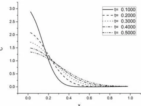
3.1. Diffusion of Material in Infinite Space without Advection
We consider an initial value problem without advection in the region −∞<x<∞ (−L<x<L in computation) with the initial condition C(x,0)=δ(x) . As a result of the symmetry, we consider the region given by 0≤x<∞ (0<x<L in computation). We summarize the conditions as follows:
Initial condition: 0 2
1 ) 0 ,
( i i
dx x
C = δ , i=0,1,⋯,N−1, (20) where δij is the Kronecker delta: δij is 1 if i= j or
0 otherwise.
Boundary condition:
(0, ) ( , )
0 , ( , ) 0 , 0
C t C L t
C L t
x x
∂ = = ∂ =
∂ ∂ (21)
0
Approximation : (0, )C t ≈C x t( , ) (22) In the case of procedure A1, we solve from (19) with
0
=
U
∑
−
= ∂
∂ =
− 1
0 0
) , ( )
, ( 2 1 ) , ( 2
N j
j j i i
t t x C t
x C t x
C α
κ ,
i=0,1,⋯,N−1, (23a)
dt
t t x C t x C dt t x
C i
i i
∂ ∂ + =
+ ) ( , ) ( , )
,
( ,
1 , , 1 ,
0 −
= N
i ⋯ . (23b) The solution of this problem is the well-known fundamental solution of the linear 1D diffusion problem:
2
4
1 ( , )
2
x t
C x t e
t
κ
πν −
= . (24)
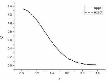
Numerical results are shown in Figs. 1 and 2. We used procedure A1 for the numerical calculation. The calculation conditions are L=1, N=20, dt=0.0005 and ν=0.089. The precision of the calculation is very high.
Figure 2. Comparison with the exact solution (t=0.5).
3.2. Diffusion of Material in Infinite Space with Advection
In the calculations in Section 3.1, we considered in the region given by 0≤x<∞ (0≤x<L in computation) using symmetry. However, since this problem is asymmetric, we must consider in the region given by −∞<x<∞ ( −L≤x<L in computation). When −L≤x<L is large enough, we can assume
( , )
0 , ( , ) 0
C L t
C L t
x
∂ ± ≈ ± ≈
∂ (25) If we consider a doublet-type initial distribution of material, the initial condition is given by
dx dx x dx x x
C( ,0)≈−δ( − 2)+δ( + 2) (26) In this case, the size and center of elements are given by
N L
dx=2 , (27a)
xi=−L+(0.5+i)dx, i=0,1,⋯,N−1. (27b) From (26), the initial condition in this case is specifically as follows:
2 2 2 21
1 1
) 0 ,
( i =− iN + iN + dx dx
x
C δ δ , i=0,1,⋯,N−1, (28) since
− < < +
≈ −
otherwise 0
2 2
in 1 ) 2
(x dx dx xN/2 dx x xN/2 dx
δ , (29a)
− < < +
≈
+ + +
otherwise 0
2 2
in 1 ) 2
(x dx dx xN/21 dx x xN/21 dx
δ . (29b)
If we adopt the explicit solution A1, we have from (19)
∑
∑
−= −
= ∂
∂ = −
− 1
0 1
0
) , ( )
, ( ) sgn( )
, ( 2
N j
j j i N
j
j j i i
t t x C t
x C dx x x U
t x
C α
κ ,
i=0,1,⋯,N−1. (30) For the check of the calculation, we use
2 2
( , ) ( , ) ( , )
( , )
( , ) 0
x x
C x t C x t C x t
dx U dx
t x x
C x t UC x t
x
κ
κ
∞ ∞
−∞ −∞
=∞ =−∞
∂ = − ∂ + ∂
∂ ∂ ∂
∂
= − + ∂ =
∫
∫
(31)
Hence, we have
const )
,
( =
∫
−∞∞C xt dx . (32) The exact solution of the problem is given byt Ut x e t Ut x
t t
x
C κ
κ πκ
4 )
( 2
2 2
1 ) , (
− −
−
= . (33)
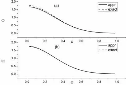
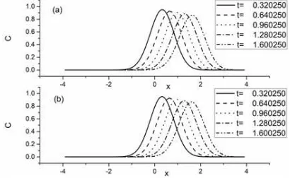
Figure 3. Space distribution of C in case of doublet type initial distribution of material: (a) approximate solution; (b) exact solution.(48)
Numerical results are shown in Fig. 3. We used A1 procedure for the numerical calculation. The calculation conditions are L=4, N=160, dt=0.0005, κ=0.089 and
0 . 1
=
U . The precision of the calculation is high.
4. Advection-Diffusion Equation in
Two-Dimension (2D)
The spatial coordinate and time are denoted as (x,y) and t, respectively. Let C(x,y,t), u(x,y,t)=u(x,y,t)i+v(x,y,t)j,
) , , (x yt
κ , and σ(x,y,t) be the material density or temperature, the advective velocity vector, the diffusion coefficient, and the material source, respectively. The 2D diffusion equation in region S is then written as
2
( ) ( )
in C
C C C C
t
S
κ σ κ κ σ
∂ + ⋅∇ = ∇⋅ ∇ + = ∇ +∇ ⋅∇ +
∂ u (34)
Rewriting (34), we have
− ∇ ⋅ ∇ − ∇ ⋅ + ∂ ∂ =
∇ κ σ
κ t C C
C
C 1 ( )
2
u . (35)
) , ( ) , ( 2
ξ x ξ x =δ
∇G , (36) and is given by
r
G ln
2 1 ) , (
π
=
ξ
x , (37)
where δ(x,ξ)=δ(x−ξ)δ(y−η) and 2 2 ) ( ) ( |
| − = −ξ + −η
= x y
r x ξ .
The fundamental solution G(x,ξ) satisfies
2 2
| |
) ( 2
1 2
1 ) , ( ) , (
ξ x
ξ x r
ξ x ξ
x ξ
x
− − = = −∇
= ∇
π π r G
G . (38)
An extension to 3D may be straight forward. Let r in 3D
be 2 2 2
) ( ) ( ) ( |
| − = −ξ + −η + −ζ
= x y z
r x ξ and the
fundamental solution be
r G
π 4
1 ) ,
(xξ =− , (39a)
3 3
| |
) ( 4
1 4
1 ) , ( ) , (
ξ x
ξ x r
ξ x ξ
x ξ
x −
− = = −∇ = ∇
π π r G
G . (39b)
And we replace area and line integrals by volume and area integrals, respectively.
From (35) and (36), we have
(
)
}
2
2
0 ( , ) ( , )
1 ( , )
( , ) ( , ) ( , )
( , ) ( , ) ( , ) ( , ) ( , ) ( , )
S G C t
C t
t C t
t t
t C t t
C t G dS
κ
κ σ
δ
= ∇
∂
− + ⋅∇
∂
− ∇ ⋅∇ −
− ∇ −
∫∫
xx
x x
x x
x ξ x
x
u x x
x
x x x
x x ξ x ξ
(40)
Hence, we obtain
(
)
( )
2 2
( ) ( , ) ( , ) ( , ) ( , ) ( , )
( , ) ( , )
( , ) ( , )
( , )
( , ) ( , ) ( , )
S S
C t G C t C t G dS
G C t
t C t
t t
t C t t dS
ε
κ
κ σ
= − ∇ − ∇
∂
+ ∂ + ⋅∇
−∇ ⋅∇ −
∫∫
∫∫
x x x
x
x x x
ξ ξ x ξ x x x ξ
x ξ x
u x x
x
x x x
(41)
where
∈ ∈ =
otherwise 0
when 2 1
when 1 )
( C
S
ξ ξ
ξ
ε , (42)
and C is the boundary of S.
We transform the integral of the first term on the right-hand side of (41). Using the vector formula:
(
)
(
)
2 2
( , ) ( , ) ( , ) ( , )
( , ) ( , ) ( , ) ( , )
G C t C t G
G C t C t G
∇ − ∇
= ∇ ⋅ ∇ − ∇ ⋅ ∇
x x
x x x x
x ξ x x x ξ
x ξ x x x ξ (43)
we obtain
( )
( , ) ( , )
( ) ( , ) ( , ) ( , )
( , ) ( , ) ( , )
( , ) ( , )
( , ) ( , )
( , ) ( , )
( , ) ( , ) ( , )
( , ) ( , )
C
S S
S S
C t G
C t G C t dl
n n
G C t G
dS t C t dS
t t t
G G
t C t dS t dS
t t
ε
κ κ
κ σ
κ κ
∂ ∂
= − −
∂ ∂
∂
+ + ⋅∇
∂
− ∇ ⋅∇ −
∫
∫∫
∫∫
∫∫
∫∫
x
x x
x x x
x x x x
x x ξ
ξ ξ x ξ x
x ξ x x ξ
u x x
x x
x ξ x ξ
x x x
x x
(44)
where n is the unit outward normal on C . Exchanging x
and ξ, we have
(
)
( , ) ( , )
( ) ( , ) ( , ) ( , )
( , ) ( , ) ( , )
( , ) ( , )
( , ) ( , )
( , ) ( , )
( , ) ( , ) ( , )
( , ) ( , )
C
S S
S S
C t G
C t G C t dl
n n
G C t G
dS t C t dS
t t t
G G
t C t dS t dS
t t
ε
κ κ
κ σ
κ κ
∂ ∂
= − −
∂ ∂
∂
+ + ⋅∇
∂
− ∇ ⋅∇ −
∫
∫∫
∫∫
∫∫
∫∫
ξ
ξ ξ
ξ ξ ξ
ξ ξ ξ ξ
ξ x ξ
x x x ξ ξ
x ξ ξ x ξ
u ξ ξ
ξ ξ
x ξ x ξ
ξ ξ ξ
ξ ξ
(45)
Removing the spatial derivatives of C(x,t) in the area integrals in (45), we have
( , ) ( , )
( ) ( , ) ( , ) ( , )
( , ) ( , ) ( , )
( , ) ( , ) ( , )
( , ) ( , )
( , ) ( , ) ( , )
( , ) ( , )
( , ) ( , )
( , )
C
C C
S S
C t G
C t G C t dl
n n
G G t
C t t dl C t dl
t n
G C t G
dS C t t dS
t t
C t
ε
κ
κ κ
κ κ
∂ ∂
= − −
∂ ∂
∂
+ ⋅ −
∂
∂
+ − ∇ ⋅
∂
+ ∇
∫
∫
∫
∫∫
∫∫
ξ
ξ ξ
ξ ξ
ξ
ξ ξ ξ
ξ x ξ
x x x ξ ξ
x ξ x ξ ξ
ξ u ξ n ξ
x ξ ξ
x ξ ξ x ξ
ξ u ξ
ξ x ξ
ξ ( , ) ( , ) ( , ) ( , )
( , ) ( , )
S S
G G
t dS t dS
t κ t σ
κ κ
⋅ ∇ −
∫∫
ξ ξ ξ∫∫
ξx ξ x ξ
ξ ξ
ξ ξ
(46)
This equation does not include the spatial derivative of the unknown variable C(x,t) in the area integrals.
If C(x,t) at IP and C(x,t) or ∂C(x,t) ∂n at BP are known from the boundary conditions, the integral representations are integral equations having unknown variables ∂C(x,t) ∂t at IP and ∂C(x,t) ∂n or C(x,t) at BP. We obtain C(x,t+dt) at IP from
t t C dt t C dt t
C(x, + )= (x, )+ ∂ (x, ) ∂ . Specifically, if C(x,0) at IP is known from the initial conditions, we can solve the initial and boundary value problems using the integral representations.
When the diffusion coefficient κ(x,t) and the advective velocity u(x,t)=u(x,t)i+v(x,t)j are given simply by
const t =κ=
κ(x, ) , (47a) const
U t = i= x
u( , ) , (47b) and (37) and (38) are substituted into (46) , we obtain
1 ( , )
( ) ( , ) ln(| |)
2
ln(| |)
( , ) 2
1
ln(| |) ( , ) ln(| |) ( , )
2 2
1 ( , ) 1 ln(| |)
ln(| |) ( , )
2 2
S S
C S
C C
C t
C t dS
t U
C t dS
U
C t n dl t dS
C t
dl C t dl
n n
ξ
ε πκ
πκ ξ
σ
πκ πκ
π π
∂
= −
∂
∂ −
−
∂
+ − − −
∂ ∂ −
− − +
∂ ∂
∫∫
∫∫
∫
∫∫
∫
∫
ξ ξ
ξ ξ
ξ ξ
ξ ξ
ξ
x x x ξ
x ξ ξ
x ξ ξ x ξ ξ
ξ x ξ
x ξ ξ
(48)
integral representation of the Poisson equation. Substituting the boundary condition into (48) and considering on the boundary C , we obtain the integral equation used in the BEM.
5. Numerical Applications to
Two-Dimensional (2D) Problems
5.1. Diffusion of Material in Infinite Space without Advection
For simplicity, we assume the conditions given in (47) and 0
=
σ . We consider the diffusion of a material placed initially at the center of the coordinates in an infinite region. In other words, the initial condition C(x,y,0)=δ(x,y) is specified in the region −∞<x<∞ and −∞<y<∞. Using symmetry, we consider only the quarter region given by
L x≤
≤
0 , 0≤y≤B.
Assuming σ(x,t)=0 and U=0, in this case, we have
(
)
2 2 0
2 2
0
2 2
0 0
1
( , , ) ( , 0, )
2 ( )
1
(0, , )
2 ( )
1 ( , , )
ln ( ) ( )
2
L B
L B
y
C x y t C t d
x y
x
C t d
x y
C t
x y d d
t
ε ξ ξ
π ξ
η η
π η
ξ η
ξ η ξ η
πν −
− +
−
+ −
∂
= − + −
∂
∫
∫
∫ ∫
(49)
where C and ∂C ∂n are assumed to be zero on the boundaries x=L and y=B.
For simplicity, we divide the region 0≤x≤L, 0≤y≤B into M×N equal elements with sides dx and dy and denote the center of each element as (xi,yj) ,
1 , , 1 ,
0 −
= M
i ⋯ , j=0,1,⋯,N−1. In other words, we have
,
L B
dx dy
M N
= = (50)
xi=dx+idx
2 , i=0,1,⋯,M−1, (51a) yj=dy+ jdy
2 , j=0,1,⋯,N−1. (51b) We summarize the initial and boundary conditions as follows:
Initial condition:
0 0 4
1 ) 0 , ,
( i j i j
dxdy y
x
C = δ δ ,
i=0,1,⋯,M−1, j=0,1,⋯,N−1. (52) Boundary conditions:
(0, , )=0
∂ ∂
x t y
C j
, j=0,1,⋯,N−1 (53a) ( ,0, )=0
∂ ∂
y t x
C i ,
1 , , 1 ,
0 −
= M
i ⋯ . (53b) Equation (49) is then approximated by the following algebraic equation:
(
)
1 2
2 2
2 0
1 2
2 2
2 0
1 1
0 0
2 2 2 2
2 2
1
( , , ) ( , 0, )
2 ( )
1
(0, , )
2 ( )
( , , ) 1
2
ln ( ) ( )
m m n
n
m n
m n
m M x dx
m x dx
m
n N y dy
n y dy n
m M n N
m n
m n
x dx y dy x dx y dy
y
C x y t C x t d
x y
x
C y t d
x y
C x y t t
x y d d
ε ξ
π ξ
η
π η
πν
ξ η ξ η
= − +
− =
= − +
− =
= − = − = = + + − − −
− +
−
+ − ∂
=
∂
⋅ − + −
∑
∫
∑
∫
∑ ∑
∫
∫
(54)
As discussed in Section 3, there are two types of solution: the explicit and implicit solutions. We use the explicit solutions below and consider the two following solutions:
Solution A1.a. Only ∂C(xi,yj,t) ∂t at IP is unknown We approximate the boundary value C(xm,0,t) and
) , , 0 ( y t
C n as follows: ) , , ( ) , 0 ,
(x t C x y0t
C m ≈ m , C(0,yn,t)≈C(x0,yn,t), (55) and the algebraic equation is approximated for
1 , , 1 ,
0 −
= M
i ⋯ , j=0,1,⋯,N−1 as
(
)
1 2
0 2 2 2
0
1 2
0 2 2 2
0
1 1
0 0
2 2 2 2
2 2
1
( , , ) ( , , )
2 ( )
1
( , , )
2 ( )
( , , ) 1
2
ln ( ) ( )
m m n
n
m n
m n
m M x dx
j
i j m x dx
m i j
n N y dy
i n y dy
n i j
m M n N
m n
m n
x dx y dy
i j
x dx y dy
y
C x y t C x t d
x y
x
C x y t d
x y
C x y t t
x y d d
η ξ
π ξ
η
π η
πν
ξ η ξ η
= − +
− =
= − +
− =
= − = − = = + + − −
−
− +
−
+ −
∂ =
∂
⋅ − + −
∑
∫
∑
∫
∑ ∑
∫
∫
(56)
The unknowns of this algebraic equation are ∂C ∂t at IP, and the number of the unknowns is M×N. The number of equations is also M×N. Hence, we can solve this equation. However, the precision is not high because of the approximation in (55).
Solution A1.b. Both ∂C(xi,yj,t) ∂t at IP, and C(xi,0,t) and C(0,yj,t) at BP are unknown
For the internal point (xi,yj) , i=0,1,⋯,M−1 , 1
, , 1 ,
0 −
= N
j ⋯ , we have
(
)
1 2
2 2
2 0
1 2
2 2
2 0
1 1
0 0
2 2 2 2
2 2
1
( , , ) ( , 0, )
2 ( )
1
(0, , )
2 ( )
( , , ) 1
2
ln ( ) ( )
m m n
n
m n
m n
m M x dx
j
i j m x dx
m i j
n N y dy
i n y dy
n i j
m M n N
m n
m n
x dx y dy
i j
x dx y dy
y
C x y t C x t d
x y
x
C y t d
x y
C x y t t
x y d d
ξ
π ξ
η
π η
πν
ξ η ξ η
= − +
− =
= − +
− =
= − = − = = + + − −
−
− +
−
+ −
∂ =
∂
⋅ − + −
∑
∫
∑
∫
∑ ∑
∫
∫
(57a)
for the boundary point on the x-axis (xi,0) , 1
, , 1 ,
0 −
= M
(
)
1 2
2 2
2 0
1 1
0 0
2 2 2 2
2 2
1 1
( , 0, ) (0, , )
2 2
( , , ) 1
2
ln ( ) ( )
n n
m n
m n
n N y dy
i
i n y dy
n i
m M n N
m n
m n
x dx y dy
i j
x dx y dy
x
C x t C y t d
x
C x y t
t
x y d d
η
π η
πν
ξ η ξ η
= − +
− =
= − = −
= =
+ +
− −
−
+ ∂
=
∂
⋅ − + −
∑
∫
∑ ∑
∫
∫
(57b)
and for the boundary point on the y-axis (0,yj) , 1
, , 1 ,
0 −
= N
j ⋯
(
)
1 2
2 2
2 0
1 1
0 0
2 2 2 2
2 2
1 1
(0, , ) ( , 0, )
2 2
( , , ) 1
2
ln ( )
m m
m n
m n
m M x dx
j
j m
x dx
m j
m M n N
m n
m n
x dx y dy
j x dx y dy
y
C y t C x t d
y
C x y t
t
y d d
ξ
π ξ
πν
ξ η ξ η
= − +
− =
= − = −
= =
+ +
− −
−
+ ∂
=
∂
⋅ + −
∑
∫
∑ ∑
∫
∫
(57c)
The number of unknowns and the number of equations are both M×N+M+N. Thus, we can solve the equation.
The exact solution of this problem is given by
t y x e t t y x
C ν
πν 4
2 2
4 1 ) , , (
+ −
= (58)
The numerical results are shown in Fig. 4. The conditions of the calculations are L=B=1, M=N=20, dt=0.0005,
5 . 0
=
t , and κ=0.089. The results indicate that Solution A.1b is more precise than Solution A1.a.
Figure 4. Numerical results at y=0.025 (t=0.5); (a) Solution A1.a; (b) Solution A1.b.
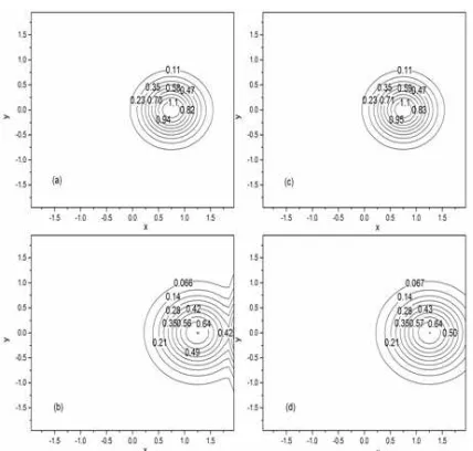
5.2. Diffusion of Material in Infinite Space with Advection
For simplicity, we assume the conditions given in (47) and 0
=
σ . We assume that the advection velocity U is not zero. In the calculations in Section 5.1, we considered in the region given by 0≤x<∞, 0≤y<∞ (0≤x<L, 0≤y<B in computation) using symmetry. However, since this problem is asymmetric, we must consider in the region given by −∞<x<∞ , −∞≤y<∞ (−L≤x<L , −B≤y<B in computation). Namely, the size and center of elements are given by
2 2
,
L B
dx dy
M N
= = (59)
xi=−L+(0.5+i)dx, yj=−B+(0.5+ j)dy,
i=0,1,⋯,M−1, j=0,1,⋯,N−1. (60) The initial and boundary conditions are as follows.
Initial condition:
2 2 1
) 0 ,
( i iM jN
dxdy x
C = δ δ ,
i=0,1,⋯,M−1, j=0,1,⋯,N−1. (61) Boundary condition:
( , )
( , ) 0 , 0
on
C t C t
x
C
∂
= =
∂
x x
(62)
C and ∂C ∂n are assumed to be zero on the boundaries L
x=± and y=±B. We have from (48)
(
)
2 2
2 2
( )
( , , ) ( , , )
2 ( ) ( )
1 ( , , )
ln ( ) ( )
2
L B L B L B
L B
U x
C x y t C t d d
x y
C t
x y d d
t
ξ
ε η ξ η
πκ ξ η
ξ η
ξ η ξ η
πκ
− − − −
− −
− + −
∂
= − + −
∂
∫ ∫
∫ ∫
ξ
(63)
The exact solution of this problem is given by 2 2
( ) 4
1 ( , , )
4
x Ut y t
C x y t e
t
κ
πκ
− + −
= (64)
We use the explicit Solution A1. The numerical results are shown in Figs. 5 and 6. The conditions of the calculations are L=B=2, M =N=41, dt=0.0005 , κ=0.089 , and
0 . 1
=
U . According to the results, the accuracy of the numerical results is high. The numerical result at t=1.25 is affected by the boundary.
Figure 6. Space distribution of C obtained by approximate and exact solutions: (a) appr., t=0.75; (b) appr., t=1.25; (c) exact, t=0.75; (d) exact, t=1.25.
6. Generalization to Generalized
Integral Representation Method
(GIRM)
6.1. Generalized Integral Representation Method (GIRM) in 1D
We introduce a generalized space fundamental solution ) , ( ~ ξ x
G defined as
) , , ( ~ ) , ( ~ ) , ( ) , ( ~ ) ,
( x t
x x G t x u x x G t x
x δ ξ
ξ ξ κ = ∂ ∂ + ∂ ∂ ∂ ∂ (65)
where δ~(x,ξ) is derived from G~(x,ξ) when G~(x,ξ) is specified. If we use the Gaussian function:
− − = 2 2 2 ) ( exp 2 1 ) , ( ~ γξ γ π ξ x x
G , (66)
then G~(x,ξ) and δ~(x,ξ) satisfy
− − − − = ∂ ∂ 2 2 3 2 ) ( exp 2 ) ( ) , ( ~ γ ξ γ π ξ
ξ x x
x x G
, (67a)
− − − = ∂ ∂ 2 2 3 2 2 2 ) ( exp 2 1 ) , ( ~ γξ γ π ξ x x x G − − − + 2 2 5 2 2 ) ( exp 2 ) ( γξ γ π ξ x x
, (67b) and x x G t x u x x G t x x t x ∂ ∂ + ∂ ∂ ∂ ∂ = ( , ) ~ ) , ( ) , ( ~ ) , ( ) , , (
~ ξ ξ
κ ξ δ x x G t x u x x G t x x x G x t x ∂ ∂ + ∂ ∂ + ∂ ∂ ∂ ∂ = ( , ) ~ ) , ( ) , ( ~ ) , ( ) , ( ~ ) , ( 2
2 ξ ξ
κ ξ κ
. (68)
Furthermore, when G~(x,ξ) is defined as (66), and
γ
tends to zero, then G~(x,ξ) and δ~(x,ξ) satisfy) , ( ) , ( ~ ξ δ ξ x x
G → , (69)
2
2 ( , ) ) , ( ) , ( ) , ( ) , , ( ~ x x t x x x x t x t x ∂ ∂ + ∂ ∂ ∂ ∂
→ κ δ ξ κ δ ξ
ξ δ x x t x u ∂ ∂
+ ( , ) δ( ,ξ), (70) where δ(x,ξ)=δ(x−ξ) is the Dirac delta function:
( , )x 0 for x and ( , )x dx 1
δ ξ = ≠ξ
∫
−∞∞δ ξ = (71)Assuming (66), G~(x,ξ) is not singular at x=ξ and decreases rapidly as |x−ξ| increases. These properties are useful in the numerical calculations. We can increase the accuracy of the numerical integration and reduce the computation time.
From (1) and (65), we have
∫
∂ ∂ − ∂ ∂ ∂ ∂ = L x t x C t x u x t x C t x x x G 0 ) , ( ) , ( ) , ( ) , ( ) , ( ~0 ξ κ
− ∂ ∂
− ( , ) (x,t) t t x C σ ∂ ∂ ∂ ∂ − x x G t x x t x
C ( , )
~ ) , ( ) ,
( κ ξ
x t dx x x G t x u − ∂ ∂ + ( , ) ~( , , ) ~ ) ,
( ξ δ ξ . (72) Rewriting (72), we have
=
∫
L dx t x t x C 0 ) , , ( ~ ) ,( δ ξ
∫
∂ ∂ ∂ ∂ − ∂ ∂ ∂ ∂− L dx
x x G t x x t x C x t x C t x x x G 0 ) , ( ~ ) , ( ) , ( ) , ( ) , ( ) , ( ~ ξ κ κ ξ
∫
∫
+ ∂ ∂ − ∂ ∂+ L L dx
x t x C x G t x u dx t x t t x C x G 0 0 ) , ( ) , ( ~ ) , ( ) , ( ) , ( ) , ( ~ ξ σ ξ . (73) Transforming the integral of the first and third terms on the right-hand side of (73) and exchanging x and ξ, we derive the generalized integral representation:
∫
L d t x t C 0 ) , , ( ~ ) ,(ξ δ ξ ξ
L x G t t C t C t x G = = ∂ ∂ − ∂ ∂ − = ξ ξ ξ ξ ξ κ ξ ξ ξ ξ κ ξ 0 ) , ( ~ ) , ( ) , ( ) , ( ) , ( ) , ( ~
[
]
∫
∂ ∂ − + == L L d t C x G t u t C x G t u 00 ( , ) ( , )
~ ) , ( ) , ( ) , ( ~ ) ,
( ξ ξ ξ
ξ ξ ξ
ξ
ξ ξξ
ξ ξ σ ξ t dξ t t C x G L
∫
− ∂ ∂ +0 ( , )
) , ( ) , ( ~
. (74) This equation does not include the spatial derivative of the unknown variable C in the integrals.
If C(x,t) at IP and C(x,t) or ∂C(x,t) ∂x at BP are known from the boundary conditions, then the generalized integral representations are integral equations with
t t x
C ∂
∂ ( , ) the unknown variables at IP and ∂C(x,t) ∂x or )
, (xt
C the unknown variables at BP. We obtain C(x,t+dt) at IP from C(x,t+dt)=C(x,t)+dt∂C(x,t) ∂t. If C(x,0) on IP is known from the initial conditions, then we can solve the initial and boundary value problem using the generalized integral representations. The generalized integral representations are equivalent to the differential equations.
When the diffusion coefficient κ(x,t) and the advective velocity u(x,t) are given simply by
const t
x =κ=
κ( , ) , (75a) const
U t x
u( , )= = , (75b) if we assume (66), (68) and (74) are given by
) , , ( ~
t xξ δ
−
− −
+
−
− −
= 2
2 5
2 2
2
3 2
) ( exp 2
) ( 2
) ( exp 2
1
γξ γ
π ξ γξ
γ π
κ x x x
−
− −
− 2
2
3 2
) ( exp 2
) (
γξ γ
π
ξ x
U x
, (76)
∫
Ld t x t C 0
) , , ( ~ ) ,
(ξ δ ξ ξ
ξ ξ dξ Gξ xσ ξt dξ t
t C x G
L L
∫
∫
−∂ ∂ =
0
0 ( , ) ( , )
~ )
, ( ) , ( ~
∂ ∂ − ∂ ∂ −
ξ ξ
κ ( , )
~ ) , ( ) , ( ) , (
~ G L x
t L C t L C x L G
∂ ∂ − ∂ ∂ +
ξ ξ
κ (0, )
~ ) , 0 ( ) , 0 ( ) , 0 (
~ G x
t C t C x G
[
G~(L,x)C(L,t)] [
UG~(0,x)C(0,t)]
U −
+ . (77)
6.2. Diffusion of Material in 1D Infinite Space with Advection
We discussed the same problem in Section 3.2. For simplicity, we assume (75) and σ=0 . We assume the triangular initial distribution of a material, and the same computation region given by −L<x<L is used. If we assume L>>1 and
( , )
0 ( , ) 0
C L t
and C L t
x
∂ ± = ± =
∂ (78)
the generalized integral representation is, from (77), given by
ξ ξ ξ ξ
ξ δ
ξ d
t t C x G d t x t
C L
L L
L
∫
∫
− ( , )~( , , ) = − ~( , )∂ ∂( , ) (79)The initial value is specified as
< ≤
−
< ≤ −
+
=
otherwise ,
0
10 0 if , 10 10
0 10 if , 10 10
) 0 ,
( L x x L
L
x L L
x L x
C . (80)
Numerical results are shown in Fig. 7. We used procedure A1 for the numerical calculation. The calculation conditions are L=4 , N=80, 160, 320 , dt=0.001, 0.0005, 0.00025,
01 . 0
=
κ , U=2.0 , and γ=0.16,0.08,0.04 . In the calculations, Nor dx was chosen assuming a proper value of the local Peclet number Udxκ , and then dt and γ were determined keeping the local Courant number
dx
Udt and the steepness of the Gaussian function dxγ constant: 0.02 and 0.625 , respectively. If N was increased, then the computational noise was eliminated, and the precise results were obtained.
Figiure 7. Space distribution of C in case of triangular initial distribution of a material: (a) approximate solution (N=80); (b) approximate solution (N=160); (c) approximate solution (N=320); (d) exact solution.
6.3. Generalized Integral Representation Method (GIRM) in 2D
In the case of 2D, the diffusion equation is given by (34), and we replace (65) by
(
κ(x,t)∇G~(x,ξ))
+(u(x,t)⋅∇)G~(x,ξ)=δ~(x,ξ,t)⋅
∇ . (81)
The extension of the theory to 3D is straightforward. We can use the Gaussian function as a generalized space fundamental solution G~(x,ξ):
−
= 2
2 2
2 exp 2
1 ) , ( ~
γ γ
π
r
Gxξ , (82)
where 2 2
) ( ) ( |
| − = −ξ + −η
= x y
r x ξ . Then, we have
− − − =
∇ 2
2 4
2 exp 2
) ( ) , ( ~
γ γ
π
r