Boundary Value Problems on Triangular Domains and MKSOR Methods

(1)

Published online June 30, 2014 (http://www.sciencepublishinggroup.com/j/acm) doi: 10.11648/j.acm.20140303.14

Boundary value problems on triangular domains and

MKSOR methods

I. K. Youssef

1

, Sh. A. Meligy

2

1

Dept. of Mathematics, Faculty of Science, Ain Shams Univeristy, Abbassia, 11566, Cairo, Egypt 2

Dept. of Engineering Mathematics and Physics, Faculty of Engineering Shoubra, Benha Univeristy, Cairo, Egypt

Email address:

[email protected] (I. K. Youssef), [email protected] (Sh. A. Meligy)

To cite this article:

I. K. Youssef, Sh. A. Meligy. Boundary Value Problems on Triangular Domains and MKSOR Methods.Applied and Computational Mathematics. Vol. 3, No. 3, 2014, pp. 90-99. doi: 10.11648/j.acm.20140303.14

Abstract:

The performance of six variants of the successive overrelaxation methods (SOR) are considered for an algebraic system arising from a finite difference treatment of an elliptic equation of Partial Differential Equations (PDEs) on a triangular region. The consistency of the finite difference representation of the system is achieved. In the finite difference method one obtains an algebraic system corresponding to the boundary value problem (BVP). The block structure of the algebraic system corresponding to four different labeling (the natural, the red- black and green (RBG), the electronic and the spiral) of the grid points is considered. Also, algebraic systems obtained from BVP with mixed derivatives are well established. Determination of the optimal relaxation parameters on the bases of the graphical representation of the spectral radius of the iteration matrices for the SOR, the Modified Successive over relaxation (MSOR) and their new variants KSOR, MKSOR, MKSOR1 and MKSOR2 are considered. Application of the treatment to two numerical examples is considered.

Keywords:

SOR, KSOR, MKSOR, MKSOR1, Triangular Grid and Grid Labeling

1. Introduction

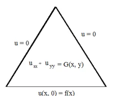
The Dirichlet problem for Poisson's equation

, , (1)

With the unknown function u given on the boundary is considered as a model problem in the numerical treatment of elliptic boundary value problems (BVP). The structure of sparse matrices obtained from the use of the finite difference method with different labeling of the grid points had encouraged many authors to work in this area [1- 7]. The successive over-relaxation method (SOR) is an important method in solving large sparse linear systems, the vital step in using the SOR method is the determination of the optimal value of the relaxation parameter ( ), [1, 2]. The introduction of the modified successive over-relaxation method (MSOR) is due to the structure of the algebraic system obtained from the red black ordering. It is common to use square mesh for such problems, but there are domains (irregular domains) [8, 9], which would include the treatment of irregular mesh points.

Figure 1. Equilateral triangular domain

However it is much simpler to use a mesh of the same shape as the region and avoid the use of irregular mesh points.

Let us consider our domain as a unit equilateral triangle as shown in figure (1). On using the finite difference method in the triangular domain as shown in figure (1), a triangle mesh of length h=1/q is superimposed [10].

2. Poisson's Equation

(2)

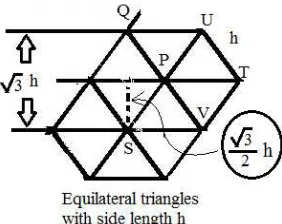
P(x, y) as shown in figure (2) and using the finite difference method in the triangular mesh, we have:

Figure 2. typical finite difference stencil

Assuming the function , is sufficiently differentiable and admits Taylor series expansions

, 2 , , √

, √ , √ , √

2 , (2)

, , , √

, √ , √ ,

√ ₂ _, ₍₃₎

And

, _√ , √ ,

√ _, √ _, √ ₍₄₎

For each mesh point (x,y) we replace Poisson's equation by the following difference equation:

, , √ , √

3 , , (5)

Where the truncation error of the above finite difference formula approximating the equation (1) at the point (i,j) can be written as:

, !

"

! " #$, % !

"

! ! , & (6)

Where ' $ ' , √ ' & ' √ (7)

Formula (6), of the truncation error guarantees the consistency of finite difference approximation with the differential equation. In the following we consider the case q=6, h=1/6, the number of internal mesh points are m=10.

3. Grid Labeling

As it was in square grid in order to write the equations in the commonly used matrix formulation () * with an

+ , + matrix ( and m-dimensional vectors ) and *

with + - - , one is forced to represent the twofold indexed unknowns by a single indexed vector

). This means that the internal grid points must be enumerated in some way. In the following we consider four ways of enumerating grid points and the corresponding matrix formulation () * for elliptic model problems as in the rectangular domains.

3.1. Natural Order Labeling

In the natural order labeling the grid points are enumerated along each row, as shown in figure (3):

Figure 3. labeling the grid points in the natural order

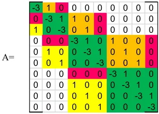
With this labeling the coefficient matrix of the linear system () * takes the form:

A= (8)

3.2. RBG Order Labeling

In the red, black and green (RBG) order labeling the grid points are enumerated such that the neighboring grid points has different label (color). If we label the points with the red points first, then the black and then the green as shown in figure (4):

Figure 4. labeling the grid points in the RBG order

With this labeling the coefficient matrix of the linear system () * takes the form:

0 0 0 0 0 0 0 0 1 -3

0 0 0 0 0 1 0 1 -3 0

0 0 0 0 1 0 1 -3 0 0

0 0 0 1 0 0 -3 0 0 0

0 0 0 0 1 -3 0 0 0 1

0 0 1 1 -3 0 0 0 1 0

0 1 0 -3 0 0 0 1 0 0

0 1 -3 0 0 1 0 0 0 0

1 -3 0 0 1 0 0 0 0 0

(3)

A= (9)

3.3. The Electronic Order Labeling

In the electronic order labeling the grid points are enumerated as shown in figure (5):

Figure 5. labeling the grid points in the electronic order

With this labeling the coefficient matrix of the linear system () * takes the form

A= (10)

The coefficient matrix in (10) appears like that in (8) of the natural ordering but the order of the diagonal blocks is reversed.

3.4. The Spiral Order Labeling

In the spiral order labeling the grid points are enumerated such that all the grid points on a peripheral circuit are grouped together as shown in figure (6):

Figure 6. labeling the grid points in the spiral order

With this labeling the coefficient matrix of the linear system () * take the form:

A= (11)

4. Elliptic Equations with Mixed

Derivatives

Partial differential equations with mixed derivative terms appear in many applications [7, 8, 9]. The treatment of mixed derivative terms introduces many problems especially on irregular domains [9]. Triangular grids give accurate representation for many domains. In the following we consider a simple elliptic equation defined on a triangular domain and introduce the structure of the linear algebraic system corresponding to the four grid labeling considered in the model problem of Poisson's equation. We introduce a formal parameter r to illustrate the correspondence of the coefficient matrices in the existence of mixed derivative term with the case without this term.

4.1. Simple Elliptic Equation with Mixed Derivative Term

We introduce the main ideas trough a simple elliptic partial differential equation of the form

, (12)

Using the difference representations in (2), (3) and (4) equation (12) can be approximated by the following difference equation:

, 1 √ , √ 1 √ ,

√ √ _, √ √ _, √ ₃ _,

, (13)

(4)

written as:

, !

"

! " #$, % !

"

! ! , & (14)

Where ' $ ' , √ ' & ' √

Using the same notations described in section (2), the structure of the coefficient matrices corresponding to the four labeling can be obtained as follows:

4.1.1. Natural Order Labeling

A= (15)

Where / √ , We note that if we put formally / 0 we obtain the matrix in (8)

4.1.2. RBG Order Labeling

A= (16)

We note that if we put formally / 0 we obtain the

matrix in (9)

4.1.3. The Electronic Order Labeling

A= (17)

We note that if we put formally / 0 we obtain the matrix in (10)

4.1.4. The Spiral Order Labeling

A= (18)

We note that if we put formally / 0 in (18), we obtain the matrix in (11)

5. Iterative Methods

Corresponding to each labeling there is a linear system of m linear equations in m unknown function values; m is the number of internal grid points (+ 1 1 10), so it can be written as a matrix equation () *

It is clear that the system has unique solution; the matrix of coefficients is diagonally dominant. Also, for large values of 2 or accordingly + the system is sparse [2].

The iterative methods for solving linear systems of algebraic equations:

We consider a linear system of m equations in the following form:

∑ 48 * ; 6 1, 2, 7 , +

9 (19)

The system (19) can be written in the matrix form as:

( * (20) Where (, is the coefficient matrix, * is a known column of constants matrix and is the unknown.

We express the matrix ( as:

( : ; ) (21) With : is a diagonal matrix with the same diagonal elements in (, and ;, ) are the strictly lower and upper triangular parts of (, respectively [2].

5.1. Successive Over-Relaxation Method (SOR)

The point SOR method for the system (19) can be written

<= ₁ <

>

?@@ * ∑ 4

<=

9 ∑8 9 = 4 < ; (22)

Where 6 1, 2, 3, 7 , + & B 0, 1, 2, 7

And C 0, 2 is a relaxation parameter, when 1 gives the Gauss-Seidel method.

Equation (22) can be written in the matrix form as

<=

DEF < G : ; : * (23)

Where _DEF G : ; # 1 G : )% is

(5)

5.2. KSOR Method [11]

The point KSOR method for the system (19) can be written

1 H <= < >H

?@@ * ∑ 4

<=

9 ∑8 9 = 4 < ; (24)

Where 6 1, 2, 3, 7 , + & B 0, 1, 2, 7

And HC I J 2, 0K, is a relaxation parameter. Equation (24) can be written in the matrix form as

<=

LDEF < 1 H G H: ; H: * (25)

Where _LDEF 1 H G H: ; G H: ) is the KSOR iteration matrix.

5.3. Modified Successive Over-Relaxation Method (MSOR)

The point MSOR method for the system (19) can be written

<= 1 < >_?M

@@ * ∑ 4

<=

9 ∑8 9 = 4 < ;

Where 6 1, 2, 3, 7 , + & B 0, 1, 2, 7

<= 1 < >_?

@@ * ∑ 4

<=

9 ∑8 9 = 4 < ;

Where 6 + 1, 7 , + & B 0, 1, 2, 7 (26)

5.4. MKSOR Method [12]

The point MKSOR method for the system (19) can be written

<= _{# =>} M

H_% < >M H

?@@ * ∑ 4

<=

9 ∑8 9 = 4 < ;

Where

6 1, 2, 3, 7 , + & B 0, 1, 2, 7

<= 1

1 H N < H

4 * O 4₉ <= O 4 <

8

9 =

P ;

Where 6 + 1, 7 , + & B 0, 1, 2, 7 (27)

5.5. MKSOR1 method [12]

The point MKSOR1 method for the system (19) can be written

<= ₁ <

4 * O 4₉ <= O 4 <

8

9 =

;

Where 6 1, 2, 3, 7 , + & B 0, 1, 2, 7

<= 1

1 H N < H

4 * O 4₉ <= O 4 <

8

9 =

P ;

Where 6 + 1, 7 , + & B 0, 1, 2, 7 (28)

5.6. MKSOR2 Method [12]

The point MKSOR2 method for the system (19) can be written

<= 1

1 H N < H

4 * O 4₉ <= O 4 <

8

9 =

P ;

(6)

<= ₁ < >

?@@ * ∑ 4

<=

9 ∑8 9 = 4 < ; (29)

Where 6 + 1, 7 , + & B 0, 1, 2, 7

6. Numerical Calculations

In this section we introduce the performance of the above mentioned six iterative methods for numerical solution of Laplace equation (Poisson's equation with G(x,y) = 0) with the four grid labeling introduced in figures 3, 4, 5 and 6 and coefficient matrices A mentioned in 8, 9, 10 and 11subject to the boundary conditions described in figure 1 with

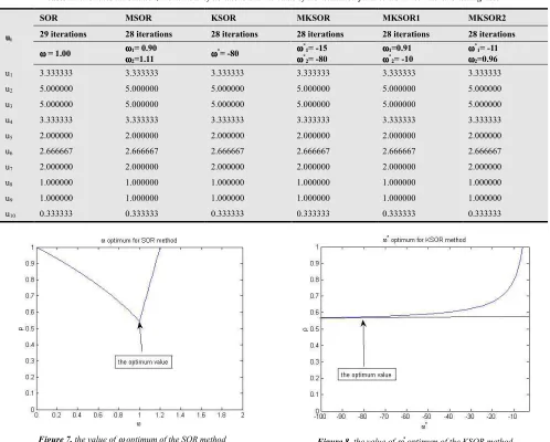
Q 36 1 . In Table 1, we summaries the results of the natural ordering with relaxation factors approximated with the help of figures 7 and 8. In Table 2 we summaries the results of the RBG ordering with relaxation factors approximated with the help of figures 9 and 10. In Table 3 we summaries the results of the spiral ordering with

relaxation factors approximated with the help of figures 11 and 12. Also, we consider equation 12 with G(x,y) = 0 with the four grid labeling introduced in figures 3, 4, 5 and 6 and coefficient matrices A mentioned in 15, 16, 17 and 18subject to the boundary conditions described in figure 1 with

Q 144#4 √3 % 1 . In Table 4 we summaries the results of the natural ordering with relaxation factors approximated with the help of figures 13 and 14. In Table 5 we summaries the results of the RBG ordering with relaxation factors approximated with the help of figures 14 and 15. In Table 6 we summaries the results of the electronic ordering with relaxation factors approximated with the help of figures 16 and 17.

The numerical solution of the Poisson's equation with natural ordering when G(x,y) = 0, u(x,0)=36x(1-x):

Table 1. illustrates the solution, the number of iterations and the value of the relaxation parameters in the natural ordering case

MKSOR2 MKSOR1

MKSOR KSOR

MSOR SOR

ui 29 iterations 28 iterations 28 iterations 28 iterations 28 iterations 28 iterations ω

ωω ω*_{1= -11} ω ωω ω2=0.96 ω

ω ω ω1=0.91 ω ω ω ω*_{2= -10} ω

ω ω ω*_{1= -15} ω ω ω ω*_{2= -80} ω

ω ω ω*_{= -80} ω

ω ω ω1= 0.90 ω ω ω ω2=1.11 ω

ωω ω = 1.00

3.333333 3.333333

u1

5.000000 5.000000

u2

5.000000 5.000000

u3

3.333333 3.333333

u4

2.000000 2.000000

u5

2.666667 2.666667

u6

2.000000 2.000000

u7

1.000000 1.000000

u8

1.000000 1.000000

u9

0.333333 0.333333

u10

Figure 7. the value of ω optimum of the SOR method _{Figure 8.}_{the value of}_ω* _{optimum of the KSOR method}

(7)

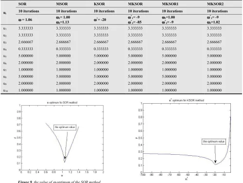
Table 2. illustrates the solution, the number of iterations and the value of the relaxation parameters in the RBG ordering case

MKSOR KSOR

MSOR SOR

ωω ω*_{1= -9} ω ωω ω2=1.02 ω

ωω ω1=1.00 ω ωω ω*_{2= -9} ω

ω ω ω*_{1= -9} ω ω ω ω*_{2= -85} ω

ω ω ω*_{= -20} ω

ω ω ω1= 1.00 ω ω ω ω2=1.13 ω

ωω ω = 1.06

3.333333 3.333333

u1

3.333333 3.333333

u2

2.666667 2.666667

u3

0.333333 0.333333

u4

5.000000 5.000000

u5

2.000000 2.000000

u6

1.000000 1.000000

u7

5.000000 5.000000

u8

2.000000 2.000000

u9

1.000000 1.000000

u10

Figure 9. the value of ω optimum of the SOR method

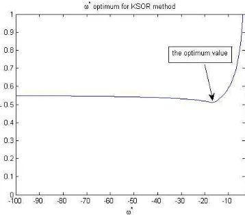
Figure 10. the value of ω* _{optimum of the KSOR method}

The numerical solution of the Poisson's equation with spiral ordering when G(x,y) = 0, u(x,0)=36x(1-x): Table 3 shows the values of u(x,y):

Table 3. illustrates the solution, the number of iterations and the value of the relaxation parameters in the spiral ordering case

MKSOR KSOR

MSOR SOR

ωω ω*_{1= -9} ω ωω ω2=1.00 ω

ω ω ω1=0.97 ω ω ω ω*_{2= -9} ω

ω ω ω*_{1= -8} ω ω ω ω*_{2= -80} ω

ω ω ω*_{= -21} ω

ω ω ω1= 0.97 ω ω ω ω2=1.13 ω

ωω ω = 1.05

3.333333 3.333333

u1

5.000000 5.000000

u2

5.000000 5.000000

u3

3.333333 3.333333

u4

2.000000 2.000000

u5

1.000000 1.000000

u6

0.333333 0.333333

u7

1.000000 1.000000

u8

2.000000 2.000000

u9

2.666667 2.666667

(8)

Figure 11. the value of ω optimum of the SOR method Figure 12. the value of ω* _{optimum of the KSOR method}

The numerical solution of the PDE equation with mixed derivative term with natural ordering when G(x,y) = 0, , 0

144#4 √3% 1 :

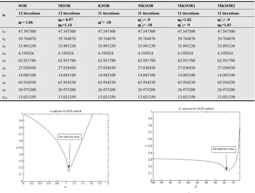
Table 4. illustrates the solution, the number of iterations and the value of the relaxation parameters in the natural ordering case (with mixed derivative term)

MKSOR KSOR

MSOR SOR

ωω ω*_{1= -7} ω ωω ω2=0.98 ω

ω ω ω1=0.96 ω ω ω ω*_{2= -8} ω

ω ω ω*_{1= -11} ω ω ω ω*_{2= -17} ω

ω ω ω*_{= -17} ω

ω ω ω1= 0.97 ω ω ω ω2=1.14 ω

ωω ω = 1.06

47.547500 47.547500

u1

65.934530 65.934530

u2

62.931780 62.931780

u3

39.764870 39.764870

u4

27.038430 27.038430

u5

35.891230 35.891230

u6

26.975200 26.975200

u7

13.021250 13.021250

u8

14.043100 14.043100

u9

4.192924 4.192924

u10

Figure 13. the value of ω optimum of the SOR method Figure 14. the value of ω

*

optimum of the KSOR method

The numerical solution of the PDE equation with mixed derivative term with RBG ordering when G(x,y) = 0, , 0

(9)

Table 5. illustrates the solution, the number of iterations and the value of the relaxation parameters in the RBG ordering case (with mixed derivative term)

MKSOR KSOR

MSOR SOR

ωω ω*_{1= -9} ω ωω ω2=1.03 ω

ω ω ω1=1.02 ω ω ω ω*_{2= -9} ω

ω ω ω*_{1= -9} ω ω ω ω*_{2= -18} ω

ω ω ω*_{= -18} ω

ω ω ω1= 0.97 ω ω ω ω2=1.14 ω

ωω ω = 1.06

47.547500 47.547500

u1

39.764870 39.764870

u2

35.891230 35.891230

u3

4.192924 4.192924

u4

62.931780 62.931780

u5

27.038430 27.038430

u6

14.043100 14.043100

u7

65.934530 65.934530

u8

26.975200 26.975200

u9

13.021250 13.021250

u10

Figure 15. the value of ω optimum of the SOR method Figure 16. the value of ω* _{optimum of the KSOR method}

The numerical solution of the PDE equation with mixed derivative term with Electronic ordering when G(x,y) = 0,

, 0 144#4 √3% 1 :

Table 6. illustrates the solution, the number of iterations and the value of the relaxation parameters in the electronic ordering case (with mixed derivative

term)

MKSOR KSOR

MSOR SOR

ωω ω*_{1= -6} ω ωω ω2=0.98 ω

ω ω ω1=1.05 ω ω ω ω*_{2= -9} ω

ω ω ω*_{1= -12} ω ω ω ω*_{2= -17} ω

ω ω ω*_{= -17} ω

ω ω ω1= 1.01 ω ω ω ω2=1.13 ω

ωω ω = 1.06

47.547500 47.547500

u1

65.934530 65.934530

u2

27.038430 27.038430

u3

62.931780 62.931780

u4

35.891230 35.891230

u5

13.021250 13.021250

u6

39.764870 39.764870

u7

26.975200 26.975200

u8

14.043100 14.043100

u9

4.192924 4.192924

(10)

Figure 17. the value of ω optimum of the SOR method

Figure 18. the value of ω* _{optimum of the KSOR method}

7. Results and Discussion

We have considered four ordering (labeling) of the grid points, the natural ordering, the red, the black and the green ordering, the electronic ordering and the spiral ordering on a triangular grid with 10 internal points.

The block structure of the coefficient matrices corresponding to the algebraic system is demonstrated. It is observed that the natural ordering (figure 3) and the electronic ordering (figure 5) give the same results (number of iterations and the values of the relaxation parameters) although the block structures on the diagonal are revised.

We find that the coefficient matrix of the linear system corresponding to the PDE with mixed derivative term contains fixed parameter (r), if we formally take / 0 we obtain the corresponding coefficient matrix of Poisson's equation for each labeling.

8. Conclusions

The number of the iterations in the RBG ordering is

considerably smaller than the other ordering similar to the red black ordering in the rectangular case in the six iterative methods considered.

The performance of the KSOR is the same as that of the SOR, provided we use the optimum value of the relaxation parameters in each case. The sensitivity of the relaxation parameters around the optimum value is more relaxed in the KSOR methods than that in the SOR methods.

The RBG ordering is the most appropriate ordering with the KSOR, MSOR, MKSOR, MKSOR1 and MKSOR2 as shown in the tables from table1to table 6.

References

[1] D. M. Young, “Iterative Methods for Solving Partial Difference Equations of Elliptic Type,” Transctions of the American Mathematical Society, Vol. 76, No. 1, pp. 92-111, Jan. 1954.

[2] D. M. Young, “Iterative Solution of Large Linear Systems,”Academic Press, London, 1971.

[3] J. W. Sheldon, “On the Numerical Solution of Elliptic Difference Equations,” Mathematical Tables and Other Aids to Computation, Vol. 9, No. 51, pp. 101 - 112, Jul. 1955. [4] B. L. Buzbee, G. H. Golub and C. W. Nielson, “On Direct

Methods for Solving Poisson’s Equations,” SIAM J. Numer. Anal., Vol. 7, No. 4, Dec. 1970.

[5] G. Birkhoff, “The Numerical Solution of Elliptic Equations,” Society for Industrial and Applied Mathematics, 1972. [6] R. A. Nicolaides, “On the Observed Rate of Convergence of

an Iterative Method Applied to a Model Elliptic Difference Equation,” Mathematics of Computation, Vol. 32, No. 141, pp. 127-133, Jan 1978.

[7] G. D. Smith, “Numerical Solution of Partial Differential Equations,” Oxford university press, 1985.

[8] S. M. Khamis, I. K. Youssef, M. H. El- Dewik and B. I. Bayoumi, “A Computational Finite Difference Treatment for PDEs Including the Mixed Derivative Term with High Accuracy on Curved Domains,” Journal of the Egyptian Mathematical Society, Vol. 17(1), pp. 15-33, 2009.

[9] I. K. Youssef, “On Strongly Coupled Linear Elliptic Systems with Application to Otolith Membrane Distortion” Journal of Mathematics and Statistics 4 (4): 236-244, 2008.

[10] D. J. Evans, “The Solution of Poisson’s Equation in a triangular region,”International Journal of Computer Math., Vol. 39 pp. 81 – 98,1991.