EVALUATION AND ANALYSIS OF GSM SIGNALS IN WARRI
U. G. Anamonye
1, G. I. Efenedo
2,*and O. M. Okuma
31,2,3DEPARTMENT OF ELECTRICAL &ELECTRONICS ENG’R,DELTA STATE UNIV.,OLEH CAMPUS,DELTA STATE.NIGERIA E-mail addresses:1[email protected], 2[email protected], 3[email protected]
ABSTRACT
This paper is aimed at comparing the signal path-loss as predicted by the Free-space model and the Okumura-Hata model with that obtained through practical measurements in the City of Warri and its environs in Delta State, Nigeria. Selected transmitting antennas mounted on base stations located at Refinery road, Enerhen junction and Okuokorkor areas were employed as the transmitters and a Lenovo A859 with received signal strength monitoring software called Net Monitor was used to measure the received signal strength at every 100 meters to a maximum distance of 1500 meters. Various path-loss models were analyzed and Free-space and the Okumura-Hata models employed in predicting the signal path-losses. The results obtained shows that the Okumura-Hata model performed well in predicting signal path-losses in Warri and its environs.
Keywords: propagation, GSM, pathloss, models, signal
1. INTRODUCTION
The importance of wireless communication is therefore not in doubt and is based on the need of man to pass information from one point to another [4]. With this in mind, we define wireless communication as the type of data communication that is performed and delivered wirelessly. This definition is all encompassing and includes any form of communication in which data in the form of voice, images, text, videos etc is delivered wirelessly from one point to another. As with every human endeavor, this means of communication did not remain in its rudimentary form. The scientific basis of wireless communication as we know it today was laid by James Clerk Maxwell and Heinrich Hertz [2]. Their research into Electromagnetic waves brought to realization the possibility of implementing wireless communication using electromagnetic waves. This possibility was tested and proved successful when Guglielmo Marconi [4] built the first complete, commercially successful wireless telegraph system that utilized radio transmission. This turned out to be the birth of wireless communication as we know it. It has since evolved from unidirection (i.e. one way transmission) to bidirectional (i.e. two way transmission) to mobile telephone systems in 1946 [10]. Due to the limitations of this system, the cellular principle was developed
where the geographical area is divided into cells. This principle was the theoretical framework upon which the Global System of Mobile Communication was developed [7]. Thanks to scientific breakthrough, the digital system of communication was developed. This brought about a major problem in the form of implementation of this system of communications. Every company involved in digital communications had their own implementations of it and this lead to compatibility problems especially in Europe where each country had its own carrier and roaming from one country to another will require you to get a new device that can work in that particular country. A standard had to be set and the European Conference of Postal and Telecommunications Administrations (CEPT) founded the Groupe Speciale Mobile and it was saddled with the responsibility of developing proposals for a pan-European Digital Mobile Communication system. The standard was finally realized and was later used as the blueprint for a global standard – the Global System for Mobile Communication (GSM) [7]. This standard has since come to dominate wireless communication despite advances in other areas of wireless communication such as Satellite Communication and Radio Broadcasting. There are three versions of GSM each using different carrier signals.
Print ISSN: 0331-8443, Electronic ISSN: 2467-8821
www.nijotech.com
The original GSM System used carrier frequencies around 900 MHZ
GSM1800 also called Digital Cellular System at the 1800 MHZ band
GSM1900 OR Personal Communication System operating on the 1900 MHZ carrier frequency and is mainly used in the USA.
As the wireless communications systems became more and more sophisticated, so did the cost of planning and implementation of this systems. This lead to the development of Radio Propagation Models also known as Channel models. They are used for the design, simulation and planning of wireless systems. These models represent important properties of propagation channels that affect the transmission of electromagnetic signals. They also help the design engineer to make changes to blueprints and analyze the cost of these changes without spending much time, money and effort [3]. An important aspect of these models is the path-loss of the propagation channel. This can be defined as the loss of energy in free space due to the conservation of energy and geometric reasons. These reasons are due to the effects of reflection, refraction, diffraction, scattering etc. [6].
2. PROPAGATION MODELS
There are several models available today that can help us calculate for path losses in line with received signal strength while taking into consideration both small and large scale effects.
2.1 COST231–Walfish–Ikegami Model
The COST 231–Walfish–Ikegami model [1] is suitable for microcells and small macrocells, as it has fewer restrictions on the distance between the base station (BS) and mobile (MS) and the antenna height. It is usually used when the distance between the MS and BS is small and the height of the MS is small as well. It has two cases. The first is for the line-of-sight (LOS) and the second is for the non-line-of-sight (NLOS). For the LOS, the path-loss, that is the loss in received signal strength is given by the formula below
PL = 42.6 + 26 log(d) + 20 log(fc) (1) In (1), d is in units of kilometers, and fc is in units of MHz for d ≥ 20 m.
For the NLOS case, the path-loss consists of the free-space path-loss L0, the multiscreen loss Lmsd along the propagation path, and the attenuation from the last roof edge to the MS, Lrts (roof-top-to- street diffraction and scatter loss) [3]:
for Lrts + Lmsd > 0, PL = PL0 + Lrts + Lmsd (2)
forLrts + Lmsd ≤ 0, PL = PL0 The free-space path-loss is:
L0= 32.4 + 20 log d + 20 log fc (3)
2.2 The ITU-R Models
For the selection of the air interface of third-generation cellular systems, the International Telecommunications Union (ITU) developed a set of models. It specifies three environments: indoor, pedestrian (including outdoor to indoor), and vehicular (with high BS antennas). For each of those environments, two channels are defined: channel A (low delay spread case) and channel B (high delay spread). The occurrence rate of these two models is also specified. The amplitudes follow a Rayleigh distribution; the Doppler spectrum is uniform between -ν max and ν max for the indoor case and is a classical Jakes spectrum for the pedestrian and vehicular environments [3]. The path-loss for both indoor, pedestrian and vehicular environments are given below
Indoor:
PL = 37 + 30 log10d + 18.3Nfloork (4) Where
K = ((Nfloor + 2) / (Nfloor + 1)) – 0.46 (5) Pedestrian:
PL = 40 log10 d + 30 log10fc+ 49 (6) Where d is in units of kilometers, and fc is in units of MHz
Vehicular:
0( – 0 ) o 0
o 2 o 0 0 ( )
2.3 The ITU-Advanced Channel Model
The ITU has defined a set of channel models for the evaluation of IMT-Advanced systems proposals. The ITU models are based on more extensive measurement campaigns (mostly done within the framework of the EU projects WINNER and WINNER 2), and cover a larger range of scenarios. The double-directional impulse response consists of a number of (delay) taps, where each tap consists of multiple rays that have different directions of arrival (DOAs) and directions of departure (DODs). The delays and angles all depend on large-scale parameters that can change from drop to drop. The following steps have to be performed in order to get the channel in a particular environment [9]:
are selected. For the mobile stations, we select locations, orientation, and velocity vectors, according to probability density functions. 2. Assign whether an MS has LOS or NLOS
according to the Table 1
3. Calculate the Path-loss according to the equations provided in the text that supplied this information. This equations cannot be made available here due to the its size [3]
2.4 The Okumura–Hata Model
Two forms of the Okumura-Hata model are available [3]. In the first form, the path-loss (in dB) is written as PL = PLfreespace + Aexc + Hcb + Hcm (8) Where PLfreespace is the Free-space path-loss, Aexc is the excess path-loss (as a function of distance and frequency) for a BS height hb = 200 m, and a MS height hm = 3 m. Hcb and Hcm are the correction factors that are provided in graphs [6].The more common form is a curve fittin of Okumura’s ori ina results. In that implementation, the path-loss is written as PL = A + B log(d) + C (9) In (9), A, B, and C are factors that depend on frequency and antenna height.
. 2 . ( ) . 2 ( ) ( ) ( 0) . . ( ) ( ) Here fc is given in MHz and d in km.
The function a(hm) and the factor C depend on the environment:
2.4.1 Small and medium-size cities ( ) ( . ( ) 0. )
( . ( ) 0. ) ( 2) C = 0
2.4.2 Metropolitan areas For f ≤ 200 MHz,
( ) .2 ( ( . )) . ( ) For f ≥ 00 MHz,
( ) .2( ( . )) . ( ) C = 0
2.4.3 Suburban environments
2 [ (
2 )] . ( ) 2.4.4 Rural area
. [ ( )] . ( )
0. ( ) The function a(hm) in suburban and rural areas is the same as for urban (small and medium-sized Cities) areas. One of the main problems with this model is the fact that it is not valid for carrier frequency above 1500MHZ. This problem is addressed by a modification which extends the region of validity from1500MHZ to 2000MHZ by redefining the following:
. . ( ) . 2 ( ) ( ) ( ) . . ( )
The value of C also changes for metropolitan areas. All values of C for other areas remain the same. i.e. C = 3 for metropolitan areas [3].
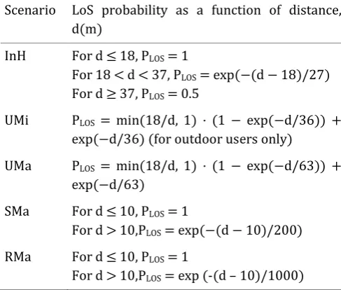
Table 1 Summary of the ITU-Advanced Channel Model Scenario LoS probability as a function of distance,
d(m)
InH For d ≤ 18, PLOS = 1
For 18 < d < 37, PLOS exp( (d )/2 ) For d ≥ , PLOS = 0.5
UMi PLOS min( /d, ) · ( exp( d/ )) exp( d/ ) (for outdoor users on y)
UMa PLOS min( /d, ) · ( exp( d/ )) exp( d/ )
SMa For d ≤ 0, PLOS = 1
For d > 10,PLOS exp( (d 0)/200)
RMa For d ≤ 0, PLOS = 1
For d > 10,PLOS = exp (-(d – 10)/1000)
2.5 Free-space Propagation Model
This model is used for predicting received signal strength when the transmitter and the receiver both have a clear, unobstructed line-of-sight. This model predict the received signal by making it a function of the distance between both the transmitter and the receiver raised to some power i.e. it is a power function [5].
Path-loss=20log10 (d) + 20log10 (f) – 27.55 (18) Here d is the distance from the Transmitting station and f is the Frequency of the Transmission
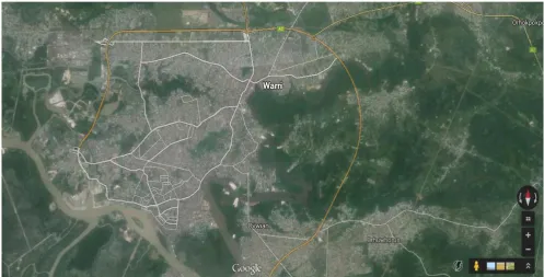
3. DESCRIPTION OF STUDY AREA
has grown from19,526 in 1933, 55,256 in 1963, 280,000 in 1980,500,000 in 1991 to 536,023 in 2006 having a high population density that is concentrated in the core areas of the city. These areas include; Warri-Sapele road, Agbassa,Okere, Okumagba Avenue, Igbudu, Iyara, Jakpa and Airport road, P.T.I. road, Udu and Ekpan. This has resulted in the area expansion of Warri metropolis reaching a size of 100 sqr. km. Studies were carried out at three major locations in Warri and environs. These locations are refinery road, Enerhen junction and Okuokorkor. Readings were taken at these locations for modeling the path losses in Warri as an urban area. According to Dijkstra and Hugo (2014),an metropolitan area is defined as a place where at least 50% of the population are living in high density clusters. Sub urban areas are places where less than 50% of the population is living in rural grid cells and less than 50% living in a high density cluster while rural areas are locations where more than 50% of the population lives in rural cell grids. A population cell grid is classified as high density if it has a density of at least 1500 inhabitants per km2 and rural if it has any population density outside of this. Looking at the city of warri and its environs, Enerhen junction which is located at the commercial nerve centre of the city fits the criteria required for urban centres. It has high rising buildings which are also clustered around the place. It also has a huge population due to its commercial and social activities which is not likely to change in the nearest
future. Fig 2 is a map showing the location of a base stations at Enerhen junction.
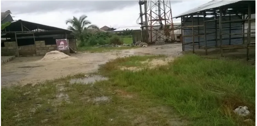
Refinery road is a sub-urban centre because it fits into the criteria stated above. It is mainly a residential area with a limited amount of commercial spots which are limited to shops and restaurants. It also has a number of hostels and a military installation. Due to its nature, its buildings are not more than two stories tall with majority of it being one story or duplexes. This location is show in figure 3 in the maps provided. Okuokorkor town was the last location taken and it has the distinction of being the only town in this study that is not located in the main city of Warri but it is one of the towns located in its environs.
The physical environment and the transmitting base station are shown in Figure 4. It is a sub-urban area based on the criteria stated above which is also visible on ground due to the low number of commercial and even residential buildings.
4. DATA COLLATION AT VARIOUS LOCATIONS
The received signal strength in dBm taking a GSM service provider as a case study for each of the locations was conducted. Interval readings of 100 meters from the nearest base station of the Provider were carried out in two days in the month of June 2015 and tabulated as presented in Tables 2, 3, 4, 5, 6 and 7.
Fig 2.Map showing the location of a base stations at Enerhen junction
Fig 3. Map showing the location of the base stations at Refinery road
Table 2. Received Signal Strength at intervals of 100 meters on DAY One at REFINERY ROAD (Provider Code 53212/1532)
Distance (m) R.S.S.1 (dBm) R.S.S.2 (dBm) R.S.S.3 (dBm) R.S.S.4 (dBm) Mean
0 -67 -70 -66 -67 -67.5
100 -51 -58 -52 -52 -53.25
200 -65 -67 -65 -63 -65
300 -67 -65 -66 -64 -65.5
400 -73 -69 -70 -69 -70.25
500 -63 -69 -67 -68 -66.75
600 -61 -67 -69 -70 -68
700 -75 -79 -76 -75 -76.25
800 -79 -71 -69 -72 -72.75
900 -76 -67 -69 -70 -70.5
1000 -73 -75 -73 -79 -75
1100 -69 -71 -65 -68 -68.25
1200 -71 -69 -68 -70 -69.5
1300 -79 -75 -71 -81 -76.5
1400 -77 -79 -78 -80 -78.5
1500 -79 -83 -81 -82 -81.25
Table 3. Received Signal Strength at intervals of 100 meters on Day 2 at REFINERY ROAD (Provider Code 53212/1532)
Distance(m) R.S.S.1(dBm} R.S.S.2(dBm} R.S.S.3(dBm} R.S.S.4(dBm} Mean
0 -63 -71 -65 -67 -66.5
100 -51 -59 -52 -52 -53.5
200 -63 -53 -57 -55 -57
300 -59 -57 -58 -59 -58.25
400 -63 -61 -68 -65 -64.25
500 -75 -67 -69 -68 -69.75
600 -71 -69 -79 -59 -69.5
700 --65 -69 -59 -70 -65.75
800 -69 -67 -65 -66 -66.25
900 -75 -73 -71 -72 -72.75
1000 -71 -69 -63 -70 -68.25
1100 -75 -77 -81 -80 -78.25
1200 -73 -77 -71 -69 -72.5
1300 -71 -69 -73 -75 -72
1400 -83 -81 -77 -79 -80
1500 -75 -77 -81 -80 -78.25
Table 4. Received Signal Strength at intervals of 100 meters on Day one at ENERHEN (Provider Code 63216/29013)
Distance(m) R.S.S.1(dBm} R.S.S.2(dBm} R.S.S.3(dBm} R.S.S.4(dBm} Mean
0 -65 -69 -66 -67 -66.75
100 -69 -68 -64 -70 -67.75
200 -81 -85 -83 -84 -83.25
300 -73 -71 -69 -73 -71.5
400 -75 -73 -70 -69 -71.75
500 -80 -82 -81 -82 -81.25
600 -79 -80 -78 -81 -79.5
700 -85 -84 -83 -86 -84.5
800 -82 -83 -81 -79 -81.25
900 -84 -85 -83 -80 -83
1000 -83 -82 -81 -85 -82.75
1100 -82 -81 -84 -85 -83
1200 -83 -84 -82 -81 -82.5
1300 -87 -87 -86 -87 -86.75
1400 -85 -86 -84 -88 -85.75
Table 5. Received Signal Strength at intervals of 100 meters on Day Two at ENERHEN (Provider Code 63216/29013) Distance(m) R.S.S.1(dBm} R.S.S.2(dBm} R.S.S.3(dBm} R.S.S.4(dBm} Mean
0 -51 -52 -55 -53 -52.75
100 -53 -51 -52 -53 -52.25
200 -51 -55 -53 -54 -53.25
300 -71 -69 -67 -65 -68
400 -71 -75 -70 -72 -72
500 -85 -79 -80 -81 -81.25
600 -79 -80 -78 -81 -79.5
700 -85 -84 -83 -86 -84.5
800 -82 -83 -81 -79 -81.25
900 -84 -85 -83 -80 -83
1000 -83 -82 -81 -85 -82.5
1100 -82 -81 -84 -85 -83
1200 -83 -84 -82 -81 -82.5
1300 -87 -87 -86 -87 -86.75
1400 -85 -86 -84 -88 -85.75
1500 -84 -85 -85 -83 -84.25
Table 6.0 Received Signal Strength at intervals of 100 meters on Day One at OKUOKOKOR (Provider Code 63217/27183)
Distance(m) R.S.S.1(dBm} R.S.S.2(dBm} R.S.S.3(dBm} R.S.S.4(dBm} Mean
0 -51 -51 -52 -55 -52.25
100 -55 -51 -53 -52 -52.75
200 -55 -51 -52 -53 -52.75
300 -53 -59 -63 -58 -58.25
400 -59 -69 -65 -67 -65
500 -71 -75 -79 -67 -73
600 -71 -67 -79 -67 -71
700 -71 -69 -75 -67 -70.5
800 -65 -69 -71 -70 -68.75
900 -71 -73 -75 -73 -73
1000 -79 -82 -81 -82 -81
1100 -81 -75 -83 -82 -80.25
1200 -80 -79 -81 -82 -80.5
1300 -82 -80 -81 -83 -81.5
1400 -83 -82 -84 -81 -82.5
1500 -84 -81 -83 -85 -83.25
Table 7: Received Signal Strength at intervals of 100 meters on Day Two at OKUOKOKOR (Provider Code 63217/27183)
Distance(m) R.S.S.1(dBm} R.S.S.2(dBm} R.S.S.3(dBm} R.S.S.4(dBm} Mean
0 -55 -52 -51 -51 -52.25
100 -52 -53 -55 -51 -52.75
200 -53 -52 -55 -51 -52.75
300 -58 -63 -53 -59 -58.75
400 -67 -65 -59 -69 -65
500 -67 -79 -71 -75 -73
600 -67 -79 -71 -67 -71
700 -67 -75 -71 -69 -70.5
800 -70 -71 -65 -69 -68.75
900 -73 -75 -71 -73 -73
Distance(m) R.S.S.1(dBm} R.S.S.2(dBm} R.S.S.3(dBm} R.S.S.4(dBm} Mean
1100 -82 -83 -81 -75 -80.25
1200 -82 -81 -80 -79 -80.5
1300 -83 -81 -82 -80 -81.5
1400 -81 -84 -83 -82 -82.5
1500 -85 -83 -84 -81 -83.25
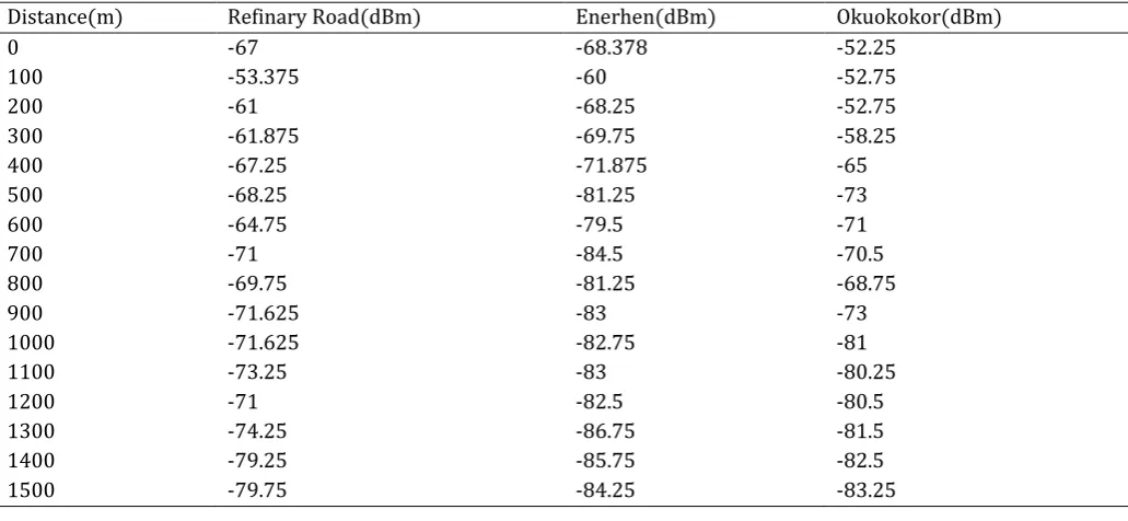
Table 8: Average signal strength for the two days in June 2015.
Distance(m) Refinary Road(dBm) Enerhen(dBm) Okuokokor(dBm)
0 -67 -68.378 -52.25
100 -53.375 -60 -52.75
200 -61 -68.25 -52.75
300 -61.875 -69.75 -58.25
400 -67.25 -71.875 -65
500 -68.25 -81.25 -73
600 -64.75 -79.5 -71
700 -71 -84.5 -70.5
800 -69.75 -81.25 -68.75
900 -71.625 -83 -73
1000 -71.625 -82.75 -81
1100 -73.25 -83 -80.25
1200 -71 -82.5 -80.5
1300 -74.25 -86.75 -81.5
1400 -79.25 -85.75 -82.5
1500 -79.75 -84.25 -83.25
5.0 COMPUTATIONAL ANALYSIS
Table 9 shows the transmitting parameters as taken in the field.
Table 9: Transmitting Antenna Parameters. Refinery
Road Enerhen Okuokokor
Antenna Heights (M) 33 20 52
Transmitting
Frequency (MHz) 900 900 900
Transmitting Power
(Watts) 40 40 40
Antenna’s Gain (dBi) 17.5 17.5 17.5
VSWR (Voltage Standing Wave Ratio)
1.5 1.5 1.5
In order for us to be able to calculate the path-loss, we have to calculate for the Effective Isotropic Radiated Power (EIRP) which is given by the formula below
( ) In (19), Pout is the transmitter power output in dBm, RL is the Signal loss in cable (dB), Gt is the Gain of the antenna (dBi)
Now:
20 o
(20) The output power which is given in watts has to be converter to Decibel milliwatts (dBm) before it can be used in the equation.
Now the path-loss (PL) is gotten as the difference between the effective Isotropic Radiated Power (EIRP) and the received power (PR) i.e
(2 )
The results obtained from equation (21) are computed in Fig 5, 6 and 7.
5.1 Path-loss using free-space model
The formula for the free-space path-loss is as shown equation 22.
20 o 20 o 2 . (22) In (22), d is distance in metres, f is the frequency of operation in megahertz of the antenna given above. Results obtained using equation 22 for modelling for free-space path-loss are in Fig 5, 6 and 7.
Okumura-Hata model, we obtained the results shown for the three locations.
( ) (2 ) . 2 . ( ) . 2 ( )
( ) (2 ) . . ( ) (2 ) In (23) to (25), fc is given in MHz and it is the
operating frequency of the antenna which is 900MHz at all the locations under study, d is in km, hm is the height of the mobile station in meters which in this case is 1m, hb is the height of the base station antenna which is 20m at Enerhen junction, 33m at Refinery Road and 52m at Okuokorkor. The function a(hm) and the factor C depend on the environment. For Refinery Road,
( ) ( . ( ) 0. )
( . ( ) 0. ) (2 ) For Enerhen Junction,
( ) .2( ( . )) . (2 ) For Okuokorkor,
( ) ( . ( ) 0. )
( . ( ) 0. ) (2 )
Having gotten the necessary parameters needed to solve for Okumura-Hata model path-loss for each of the locations. Graphs in Fig 5,6 and 7 are the modelled outputs.
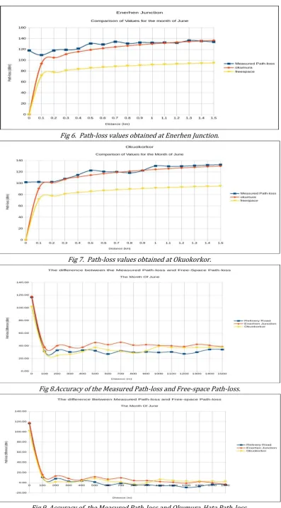
Analyzing output curves in graphs Fig 6 -12 shows that there is a general increase of path-loss with respect to distance. This increase however is not strictly linear as values closer to the base station are larger than those father from it. This is due to the uneven distribution of substances that can increase
the path-loss of the signal. At Enerhren junction, we find that the path-loss was already above 130dBm at a distance of 700 m from the base station with a variation of + 4dBm for each subsequent increase of about 100 m till we get to 1500 m. At refinery road, the results obtained is generally lower than that obtained at enerhen junction with the maximum path-loss obtained being 129dBm but this result was still subject to the exact type of variations that occurred with the previous case with the values hovering around 120 dBm for much of the distances covered. Finally, the maximum values obtained for Okuokorkor was similar to Enerhen junction but this values was not constant until we were at distances above 1100 m.
Table 13 results show that irrespective of the environment, the results obtained for the predicted path-loss values would always be the same. This results also shows that for the specified maximum distance which is 1500 m the predicted path-loss would always be the same for the three locations which is 95.06 dBm. It is also observed from the results above that there is a gradual increase in the predicted path-loss with each increase in distance. That is as we increase the distance, the predicted path-loss must increase. This is due to the fact that the predicted path-loss is a function of transmitting frequency and distance and since the transmitting frequency is the same, the change is as a result of change in distance only. When we compare the two path-losses with respect to Measured path-loss, the results obtained are shown in graphs in Fig. 5, 6 and 7.
Fig 6. Path-loss values obtained at Enerhen Junction.
Fig 7. Path-loss values obtained at Okuokorkor.
Fig 8.Accuracy of the Measured Path-loss and Free-space Path-loss.
Fig 5 shows us that the Okumura-Hata model was fairly accurate at predicting the Path-loss to be expected at this location. Comparing it with the Measured Path-loss, the result shows us that both values intersects at more than four points with the other Measured values being either above or below the values predicted by the Okumura-Hata model. The Free-space model on the other hand was very far from the measured values. The graph of the values obtained at Enerhen junction is presented in Fig 6. From Fig 6, both lines representing the measured values and the Okumura-Hata model intersected at different points with the remaining values being very close. This is obvious that the measured values settles for the predicted values obtained from the Okumura-Hata model as the range of the distance is increased. It is also obvious that the Free-space model is still not performing well when compared with the other two method. Lastly, the graphical representation of the values obtained at Okukorkor is presented in Fig 7. The curves of Fig 7 show that the Okumura-Hata model still maintained its high performance and integrity. It was still very close to the measured value, ignoring the fact that they both intersected at a single point. The Okumura-Hata model performed well in trying to predict the path-loss in this area. In general, the Okumura-Hata model performed well in trying to predict the Path-loss in Warri and its environs.
6. FINDINGS
Firstly, we discovered that the Okumura-Hata model was very good at giving a good estimate of the path-loss at the areas under consideration. The accuracy of the Okumura-Hata model path-loss (Fig 8 and 9) gotten through the modellings when compared with the free-space only got better as the distance from the base station is increased. It is also very close to the measured path-loss obtained from measurements. This shows us that the Okumura-Hata model can be used as an alternative to calculate for the path-loss in thisareas. Secondly, it was observed that the measured path-loss, as seen from the graph, usually settles for the same value as the Okumura-Hata model as the distance increases. This also adds to the already high reliability of the Okumura-Hata model. Lastly, the free-space model was shown to be highly unreliable as shown in the graphs shown in figure 8. This model did not predict any value close to the measured or Okumura-Hata values. This shows that the Free-space model cannot be relied upon at any distance or in any environment to accurately predict the signal path-loss.
7. CONCLUSION AND RECOMMENDATIONS
In line with the aim of this study, it has been proven practically, through these findings, that the
Okumura-Hata model is very accurate in its prediction of the path-loss in Warri and its environs. These findings also showed that the free-space model is very inaccurate in its prediction of the path-loss experienced in Warri. It is to be noted that despite the accuracy of this model in predicting the path-loss in this environment, the results obtained in this research is subject to changes due to the ever changing nature of our environment. These changes can be natural or man-made, permanent or temporary, instant or gradual. It should also be noted that these two models are not the only models that can be used to predict the path-loss in an environment like Warri. The Okumura-Hata model has proven to be very reliable and accurate in its prediction of path-loss encountered and it is recommended as a suitable replacement to taking exact measurements if the cost in time, money and effort is too great to bear. We however made the following recommendations:
1. That further research be carried out in Warri and its environs, comparing the accuracy of other prediction models and comparing it with that of the already established Okumura-Hata model.
2. We recommend also that the readings acquired during the cause of this study be reassessed after a couple of years due to the ever changing nature of the environment as stated above.
3. The Free-space model should not be used as the major prediction model in any practical work.
8. REFERENNCES
[1] Afo ayan J,, Obot A and Simeon O “Comparative ana ysis of path loss prediction models for urbanmacrocellular environments”, Nigerian Journal of Technology, Vol. 30, No. 3, 2011.
[2] Andrea Go dsmith, “ ire ess Communications,” Cambridge University Press,
[3] Andreas F. Molish, “ ire ess Communication,” John Wiley & Sons Ltd, The Atrium, Southern Gate, Chichester, West Sussex, PO19 8SQ, United Kingdom, 2011.
[4] Daniel K. on , “Fundamentals of Wireless Communication Engineering Technologies,” John i ey & Sons, Inc., Hoboken, New Jersey, 2012.
[5] Isabona Joseph, Konyeha. C. C, Chinule. C. Bright, and Isaiah Gre ory Peter, “Radio Field Strength Propagation Data and Path-loss calculation methods in UMTS Network”, 2013.
[6] Nasir Faruk, Adeseko A. Ayeni and Yunusa A. Adediran, ”On the study of empirical path loss modelsfor accurate prediction of signal for secondary users”, Progress In Electromagnetics Research B, Vol. 49, 155–176, 2013.