R E S E A R C H
Open Access
Stochastic optimization model of
aquacultured fish for sale and ecological
education
Hidekazu Yoshioka
1*and Yuta Yaegashi
2*Correspondence: [email protected] 1Faculty of Life and Environmental Science, Shimane University, Nishikawatsu-cho 1060, Matsue, Shimane 690-8504, Japan Full list of author information is available at the end of the article
Abstract
A stochastic optimization model for management of aquacultured fish for sale and ecological education is established. Population dynamics of the fish is described with a system of stochastic differential equations assuming that they are stochastically harvested after an opening time: the variable to be optimized. A remarkable difference between the present and conventional models for the aquaculture is that the former considers the harvesting for ecological education, which is a key for current inland fishery especially in Japan. Finding the cost-effective optimal opening time effectively reduces to solving an algebraic equation. Mathematical analysis on the optimal opening time clearly reveals its unique existence and qualitative behavior, such as its dependence on the model parameters, which have practical implications. A demonstrative application example of the model is also presented focusing on an aquaculture ofPlecoglossus altivelisin Japan.
Keywords: aquaculture; population dynamics; stochastic differential equation; Poisson process; fisheries cooperatives; ecological education
1 Introduction
Aquaculture is one of the most profitable fisheries sectors that conventionally farms, har-vests, and sells fishery resources []. Cost-effective and sustainable management strategies for aquaculture have been studied from both scientific and engineering viewpoints. Clarke et al. [] reviewed fish vaccine development using plant genetic engineering techniques for sustainable aquaculture. Mazid et al. [] investigated cost-effective feeding strategy for aquacultured fish using locally available ingredients.
Population dynamics models can efficiently simulate behavior and dynamics of aquatic organisms [–]. For modeling the dynamics related to aquaculture, stochastic models turned out to be able to compute cost-effective, environmentally- and/or ecologically-sound management strategies of fishery resources under a variety of conditions [–]. Stochastic differential equations (SDEs) [] have served as one of the most important tools for optimization problems in aquaculture because of their power to effectively han-dle population dynamics subject to uncertainties. Nøstbakken [] numerically computed optimal management rules of aquaculture systems subject to regime-switching stochastic stocks and prices of farmed fishes. Reed and Clarke [] derived optimal harvesting and pricing rules for aquacultured fishes with the stochastic and size-dependent growth rate.
León-Santana et al. [] analytically derived formulae to achieve environmentally-sound aquaculture based on linear SDEs.
Inland fishery resources, many of which are aquacultured, have long been of central im-portance as food sources of humans [, ]. Currently, establishment of adequate manage-ment policies for aquacultured fishes is an urgent issue for inland Fisheries Cooperatives (FCs) because of their severe financial and operational difficulties, which are considered due to decrease of the fish catches and aging of officers. Recently, the authors proposed de-terministic [] and stochastic [] optimization models to achieve cost-effective manage-ment of artificial aquaculture systems (pools). Their models can find the optimal opening (stopping) time [], which gives the most cost-effective management strategy of aquacul-tured fishes. The models, however, lack one important factor in the aquaculture of inland fishery resources that some FCs have to manage harvesting not for sale. The most impor-tant purpose of the harvesting not for sale is the ecological education [, ]. Actually, each FC in Japan has a duty of ecological and environmental conservation and education around the river where it authorizes []. Some FCs in Japan harvest aquacultured fishes for the exchange meetings of ecological education where local residents and their children learn about and enjoy ecology and environment of neighboring rivers []. For example, the harvested fishes are used for catching competition of the fishes by the children of local residents in exchange meetings (Figure ). Through the ecological education, FCs teach about the fishes they farm and aquatic organisms living in their river. Throughout com-munications between the authors and an FC in Japan during -, we found that the effect of ecological education should be considered in optimization models of aqua-cultured fishes of FCs in Japan, in which fishes are harvested for both sale and ecological education. Furthermore, we also found that FCs consider that the ecological education can be a critical factor to continue inland fishery sustainably. However, to the authors’ knowl-edge, such mathematical modelling of an aquaculture considering the harvesting not for sale, despite its importance, has not been carried out so far. This is the strong motivation for writing this paper.
The purpose of this paper is to develop a new, tractable stochastic process model for aquaculture considering the harvesting not for sale, which can be utilized for decision-making of the cost-effective and ecologically conscious aquaculture. Stochastic popula-tion dynamics in an artificial aquaculture system is described with a system of SDEs that govern the total number of the population and its representative weight. The opening time of harvesting is set as the variable to be optimized. The decision-maker in our optimiza-tion problem is the manager of an FC. The opening time is optimized by the manager so
that the performance index, which is a net profit by the aquaculture, is maximized. The main difference between the present and conventional models [, –] is that fishes are harvested not only for sale but also for ecological education to local residents. This effect is incorporated into both the population dynamics model and the performance in-dex. Mathematical analysis on the optimal opening time is carried out and its results are verified with numerical computation focusing onPlecoglossus altivelis, which is one of the most important inland fishery resources in Japan, managed by Hii River Fisheries Cooper-ative (HRFC). This paper is the first attempt to model aquaculture considering harvesting for ecological education.
The rest of the paper is organized as follows. Section presents the mathematical model for cost-effective management of aquacultured fishes without reproduction. Section presents mathematical analysis results on the model. Section performs numerical com-putation to verify the mathematical analysis results with an application toPlecoglossus al-tivelis(Ayu), which is an important inland fishery resource in Japan. Section concludes this paper and presents future perspectives of our research.
2 Methods: mathematical model
The population dynamics model in this paper is not significantly different from the con-ventional ones [] except for that it is driven by Poisson noises. On the other hand, the performance index to be maximized, which has a term on profit by harvesting the fish for ecological education, distinguishes the present model from the conventional ones. Here-after,a∧bfora,b∈Rrepresents the smaller value betweenaandb.
2.1 Governing equations
The time is denoted ast∈[,T] wheret= ,T are the initial and terminal times of an aquaculture, respectively. The fish is introduced into the system only att= . The pop-ulation dynamics in an artificial aquaculture system is reasonably considered to be non-renewable []. The dynamics is described with the representative (average) weight of in-dividualsWt≥ and the total number of individualsNt≥. The governing equations
ofWt andNt are assumed to be independent with each other. This is a reasonable
as-sumption for realistic aquaculture system operated by well-experienced managers with a controlled, sufficiently large pool. The representative weightWtmonotonically increases
throughout the period. On the other hand, the total number of individualsNt
monotoni-cally decreases at the same time. All the stochastic integrals in what follow are defined in the Itô’s sense [].
exchange meetings are held during [τ,T), which is also modelled as a Poisson processP()t
with the intensityλ()> . The total number of potentially harvested individuals for eco-logical education at the timetfollows a non-negative continuous-time stationary Markov processc()t . Scheduled date and time of each exchange meeting are usually determined
beforet= , but they are possibly held on different date and time due mainly to climate stochasticity. The mean values of c()t andc()t are assumed to exist and are denoted as
C()> andC()> , respectively. The stochastic processesP()
t ,P()t ,c()t , andc()t are
as-sumed to be independent with each other. The stochastic population dynamics is consid-ered under usual filtration generated by the processesPt(),P()t ,c()t , andc()t as in the
con-ventional stochastic process models. Mathematical properties and applications of Poisson processes are presented in Ross [].
The initial conditions ofWt andNt at the timet= are assumed to be given as
non-negative numbers. The governing equation ofWtis given by
dWt
dt =Wtg(Wt), t> ()
with the growth rateg. This paper assumes the constantg=r> or the generalized Ver-hulst model (theta-logistic model) given as []
g(w) =r
–
w K
θ
, w≥ ()
with the intrinsic growth rater> , the maximum body weightK> , and the nonlinearity parameterθ> . This model is more realistic than that withg=rsince the latter gives un-bounded exponential growth. Settingθ= in () yields the conventional Verhulst model. Behavior of solutions to the generalized Verhulst model and its related models has been investigated in detail [, ].
Denote the natural mortality rate of the fish asR. The governing equation ofNtis given
by the SDE
dNt= –RNtdt–χ{t≥τ}
n=
c(tn)dP(tn), t> , ()
which is explicitly solved with stochastic integrals (Chapter of []) as
Nt=
⎧ ⎨ ⎩
Nexp(–Rt) (≤t<τ),
Nexp(–Rt) –
n=
t
τexp(–R(t–s))c
(n)
t dP(tn) (τ≤t≤T),
()
whereχ{t≥τ}is the indicator function such thatχ{t≥τ}= fort≥τandχ{t≥τ}= otherwise.
Hereafter, E[·] represents expectation. The mean E[Nt] is calculated as
E[Nt] =
⎧ ⎨ ⎩
Nexp(–Rt) (≤t<τ),
exp(–R(t–τ))[Nexp(–Rτ) –B(exp(R(t–τ)) – )] (τ≤t≤T)
()
2.2 Performance index
The performance index that quantifies optimality of each management strategy is es-tablished from the viewpoint of the manager of an FC as the decision-maker. The per-formance index consists of (statistically) known variables and parameters so that the decision-maker can choose a strategy before they start an aquaculture. We then assume that the decision-maker can predict the (mean) extinction timeTexof E[Nt]:
Tex=inf
t|E[Nt] = ,t≥
. ()
This assumption is natural under the situation where the decision-maker can empirically predict laws of the stochastic processesPt(),P()t ,c()t , andc()t , but not their paths. It is then
reasonable to give the performance index, which is net benefit of the FC by the aquacul-ture, as an expectation of a functional of stochastic processes. The present performance index assumes a situation where the population is stochastically harvested with fluctuating demands.
The present performance index is formulated as an extended, stochastic counterpart of that in Yoshioka and Yaegashi []:
Jτ= E
T∧Tex
τ
α()c()t WtdP()t +
T∧Tex
τ
α()c()t WtdPt()–
T∧Tex
βpNtWtdt
, ()
whereα(),α(), andβare positive weight parametersa prioridetermined by the manager, andpis the cost of farming the fish per unit time. As presented in (), the performance index consists of the three terms. The first term is the profit by selling the fish during the period [τ,T]. The second term is the profit by providing the fish for exchange meetings for ecological education during the period [τ,T]. The second term is possibly difficult to financially evaluate. This term indirectly represents the profit by the exchange meetings. Officers of HRFC consider that harvesting the aquacultured fish for ecological education can indirectly lead to conservation of environment and ecology of rivers by local residents, which consequently becomes beneficial for the FC. Finally, the third term is the cost of farming the fish during the whole period [,T], which involves feeding cost of the fish and cleaning cost of their excrements in the pool, both of which would be larger for larger total biomassNtWt. As described above,Jτ is not purely monetary one whose weights
involve the attitude of the decision-maker. Importance of each term can be modulated by the decision-maker based on his/her consideration that which term is of importance for the FC. Therefore, different FCs would have different values of the weight parameters.
SinceJτ is a function of the opening timeτ∈[,T], and it is continuous with respect to
τ, there exists at least one maximizerτ=τ∗ofJτ such that
τ∗= arg max
τ∈[,T∧Tex]
Jτ. ()
3 Mathematical analysis
Mathematical analysis on existence and uniqueness of the optimal opening timeτ∗is car-ried out. A primitive stochastic process model is also analyzed in this section. Practical implications of the mathematical analysis results are presented as well, which are verified numerically in the next section.
3.1 Primitive model
Theoretical behavior of a primitive population dynamics model is briefly studied in order to get insights on the behavior of the presented model. Letkbe a fixed natural number. LetP(tn)(n= , , . . . ,k) be independent Poisson processes with the intensities ofλ(n)> .
The amplitude ofP(tn)is modulated by the stationary and continuous-time non-negative
stochastic processc(tn)having the mean valueC(n). The processesPt(n)andc(tn)are assumed
to be independent with each other. Consider the primitive model that governs a stochastic processMt:
dMt= –RMtdt– k
n= c(tn)dP
(n)
t , t> . ()
The SDE is subject to the initial conditionMat the initial timet= . The SDE () can be solved as
Mt=Mexp(–Rt) –
t
exp–R(t–s)
k
n=
c(sn)dP(sn), t> . ()
SinceP(sn)andc(sn)are independent, the mean E[Mt] is calculated as
E[Mt] =Mexp(–Rt) – E
t
exp–R(t–s)
k
n=
c(sn)dPs(n)
=Mexp(–Rt) –
t
exp–R(t–s)
k
n=
Ec(sn)λ(n)ds =exp(–Rt)M–A
exp(Rt) – , t> , ()
with
A=
k
n=
C(n)λ(n). ()
The extinction timeTex,ofMtis defined as
Tex,=inf
t|E[Mt] = ,t≥
, ()
which is exactly calculated as follows by (). The extinction timeTex,is calculated as
Tex,= Rln
+M A
= Rln
+M
k
n= C(n)λ(n)
–
Remark . The variance of the processMtis explicitly expressed for somec(tn), although
it has less simpler expression than that of the mean value (). Assume that eachc(tn)follows
a Cox-Ingersoll-Ross (CIR) model []
dc(tn)=a(n)
C(n)–c(tn)
dt+σ(n)
c(tn)dB(tn), t> , ()
subject to the initial condition c(n) =C(n) where a(n) > and σ(n) ≥, and B (n)
t (n=
, , . . . ,k) are standard -D Brownian motions independent with each other. For a pos-itive initial condition, the process is strictly pospos-itive if []
a(n)C(n)>σ(n), ()
which is assumed throughout this paper. The CIR model is a minimal model that has a stationary distribution with exact mean and variance [, ]. Assume that the process ct(n)satisfiesc(n)=C(n). Then, the mean and variance ofc
(n)
t fort> are E[c(tn)] =C(n)and
Var[c(tn)] = C(n)(σ(n))
a(n) , respectively. Actually,c (n)
=C(n)is a possible candidate of the initial condition, but may not be realized in practice. For the sake of simplicity of mathemati-cal analysis, the mean value of the processc(tn), which is weak stationary and has a finite invariant measure, can be approximated byC(n). A similar treatment is applied to the vari-ance ofc(tn). This approximation does not significantly affect the numerical analysis results
presented later because of the conditiona(n)T where the influences of the initial con-dition rapidly decay. By (), the varianceVar[c(tn)] is bounded from above as
Varc(tn)
=C (n)(σ(n))
a(n) <
C(n)=Ec(tn)
. ()
The variance of the processMt is then exactly calculated with the help of the isometry
formula for Poisson processes (Chapter of []). The exact expression of the variance ofMtis presented in Appendix , which is utilized in Section .
3.2 Existence and uniqueness of optimal opening time
Existence of the optimal opening timeτ∗, which is a maximizer of the performance index Jτ, is mathematically analyzed. Several auxiliary results for analyzingτ∗ are firstly
pre-sented. By (), the extinction timeTex=Tex(τ) forNtis given as follows. The extinction
timeTex=Tex(τ) forNtis
Tex=τ+ Rln
+Nτ B
=τ+ Rln
+Nexp(–Rτ) B
. ()
A straightforward calculation shows that the first- and second-order derivatives ofTex= Tex(τ) with respect toτ are
dTex dτ =
B B+Nexp(–Rτ)
, <dTex
dτ < ()
and
dT ex dτ =R
dTex dτ
–dTex dτ
= BRNexp(–Rτ) [B+Nexp(–Rτ)]
respectively. Therefore,Texis convex and increasing with respect toτ. Equation () leads toTex(τ)≥Tex() forτ ≥, showing thatTex(τ)≥T forτ≥ ifTex()≥T. Therefore, Tex≥Tif
N≥B
exp(RT) – . ()
The inequality () means that there are remaining individuals at the terminal timeT when sufficiently large number of the individuals are introduced into the system.
It is shown below that behavior of the optimal opening timeτ∗is qualitatively different between the exclusive casesTex≥T andTex<T. In both cases, the performance indexJτ
can be rewritten as
Jτ =
T∧Tex
τ
λ()α()C()Wtdt+
T∧Tex
τ
λ()α()C()Wtdt
–
T∧Tex
βpE[Nt]Wtdt
=A˜
T∧Tex
τ
Wtdt–βp
T∧Tex
E[Nt]Wtdt ()
withA˜=λ()α()C()+λ()α()C(). The first-order of partial derivative ofJ
τ with respect to
τ is calculated as (Appendix )
dJτ
dτ = –
˜
AWτ+βpBR
T
τ
exp–R(t–τ)Wtdt
< ()
forTex≥T. ddJττ is calculated as
dJτ
dτ =A˜(Fτ–ηGτ) ()
forTex<T. Here,
Fτ =
dTex
dτ WTex–Wτ ()
and
Gτ=
Tex
τ
exp–R(t–τ)Wtdt ()
withη=βpBR˜
A .
The equation () immediately gives the following proposition sinceJτis monotonically
decreasing with respect toτ whenTex≥T. Define the critical opening timeτexas
τex=inf
τ≥|Tex(τ)≥T
. ()
The critical opening timeτexis the unique positive solution to
T=Tex(τex) =τex+ Rln
+Nexp(–Rτex) B
when the condition () does not hold, which certainly exists by () and (). In addition, <τex<T. On the other hand,τex= if (). From a mathematical viewpoint, it is impor-tant to remark thatτ∗≤τexwhenTex≥T,J∈C([,T∧Tex])∩C(,τex)∩C(τex,T∧Tex),
τ∗= when (). The conditionτ∗≤τexwhenTex≥Tshows that it is optimal to setτ∗= ifNis too large. Although this is theoretically optimal for such a case, it has not been em-ployed in conventional aquacultures. Therefore, this strategy is not reasonable from the viewpoint of managing fishery resources. We thus assume that the condition () is not satisfied in what follows. The mathematical analysis below focus on the caseTex<T. The possible range ofτ∗is then [,τex]. In the above-mentioned sense,τexis an upper bound ofτ∗.
A sufficient condition forτ∗> , which is consistent with the actual strategies for manag-ing aquaculture systems by FCs, is presented below. Practical implications of the condition are presented as well.
Proposition . τ∗> if
dTex()
dτ WTex()–W>η
Tex()
exp(–Rt)Wtdt. ()
Proof τ∗> if dJτ
dτ|τ=> sinceJτ is continuously differentiable with respect toτ ≥.
Substituting () and () into dJτ
dτ|τ=> leads to () sinceA˜> .
Based on Proposition ., the conditions to guaranteeτ∗> for several growth models are derived.
Proposition . For g=r(= const) > ,the condition()is satisfied for sufficiently large r andη–.
Proof The condition () is satisfied if its left-hand side is positive andηis sufficiently small. The latter is always possible because the parametersp,β,α(), andα()involved in
ηdo not appear in the left-hand side of (). Actually, choosing sufficiently smallpβ or sufficiently largeA˜=λ()α()C()+λ()α()C()can achieve arbitrary small and positiveη.
SinceWt=Wexp(rt) in the present case, the left-hand side of () becomes dTex()
dτ WTex()–W=
B B+N
WTex()–W=
+N B
r
R– –
W. ()
The right-hand side of () becomes
η
Tex()
exp(–Rt)Wtdt=
ηW r–R
–exp–RTex()
<ηW
r–R ()
ifr>R. The condition () is thus satisfied if
+N B
r
R– > ηW
r–R, ()
Proposition . then leads to the following theorem for the generalized Verhulst model:
Wt=
Kθ
(KθW–θ
– )exp(–rθt) +
θ
, ()
which behaves for sufficiently smallWK–as
Wt∼
K
(KθW–θ
– )
θ
exp(rt). ()
Theorem . For the generalized Verhulst model,the condition()is satisfied for suffi-ciently large r and suffisuffi-ciently small WK–andη.
Proof Following the proof of Proposition ., to prove the proposition, it is sufficient to show that the left-hand side of () can be made positive for sufficiently largerand suffi-ciently smallKW–
. By () and (), the left-hand side of () is evaluated as
dTex()
dτ WTex()–W∼
K
(KθW–θ
– )
θ
+N B
r
R– –
. ()
On the other hand, the right-hand side of () is evaluated as
η
Tex()
exp(–Rt)Wtdt<
ηK R
–exp–RTex()
<ηK
R . ()
Therefore, the condition () is satisfied if
η
R<
(KθW–θ
– )
θ
+N B
r
R– –
, ()
which holds true for sufficiently largerand sufficiently smallWK–andη.
Remark . Proposition . and Theorem . show that the optimal opening timeτ∗is positive, which is in accordance with the reality, if the aquacultured fishes grow sufficiently fast and large and the demand of harvesting them is sufficiently large. A practical implica-tion of the analysis results on management of aquacultured fish is that the decision-maker should carefully observe their growth. Similar results have been theoretically derived in Yoshioka and Yaegashi [] using a different population dynamics model based on an op-timization approach. This fact implies that there exists an underlying universal principle for cost-effective management of aquacultured fish harvested at a certain rate after an opening time.
Uniqueness results ofτ∗for smallpare finally presented in this sub-section. Key propo-sitions for the casep= , which seem to be not reasonable from a practical viewpoint but actually serve as the basis for dealing with the case with sufficiently smallp> , are presented below.
Proof By () andη= ,
dJτ
dτ =AF˜ τ =A˜
dTex
dτ WTex–Wτ
, ≤τ<τex. ()
By () and (), () is rewritten as
dJτ
dτ =AW˜
dTex dτ
exp(r–R)(Tex–τ)
– exp(r–R)τ, ≤τ<τex, ()
showing
sgn
dJτ
dτ
=sgn{r–R}. ()
Therefore, by (),τ∗is determined uniquely as
τ∗=
⎧ ⎨ ⎩
(r<R),
τex (r>R).
()
Proposition . Assume p= ,g is given by the generalized Verhulst model()with r>R andθ≥.Then,τ∗∈[,τex]exists uniquely.
Proof In this case,η= as in Proposition . and
dJτ
dτ =A˜
dTex dτ exp
(r–R)Tex
WTexexp(–RTex) –Wτexp(–Rτ)
, ≤τ<τex ()
by () and (). In addition,
dJ
τ
dτ < ()
whenτ =τ∗∈(,τex) exists (Proposition A. in Appendix ). Therefore,Jτ does not have
local minimum in (,τex). This follows thatτ∗∈[,τex] is determined uniquely with the help of the classical intermediate value theorem as
τ∗=
⎧ ⎪ ⎪ ⎨ ⎪ ⎪ ⎩
(ifF≤),
˜
τ (ifF> ,Fτex< ),
τex (ifF> ,Fτex≥),
()
whereτ˜is the unique solution ofFτ= .
Now, an application of the classical implicit function theorem with the smoothness of Fτ–ηGτ with respect toτandpimmediately shows the following unique existence
theo-rem ofτ∗∈(,τex) such that ddJττ for smallp> .
Theorem ., although it can effectively characterizeτ∗∈(,τex), is possibly not sharp as the numerical computation results demonstrate later.
3.3 Comparative statics of the critical and optimal opening times
Comparative statics of the critical opening timeτexand the optimal opening timeτ∗such that <τ∗<τex, namely their dependences on model parameters, is carried out. The com-parative statics ofτexis firstly carried out. A straightforward calculation shows the follow-ing proposition.
Proposition . The critical opening timeτexsatisfies
∂τex
∂R =
RB(T–τex)
B+Nexp(–Rτex)
+Nτex
RB exp(–Rτex) > , ()
∂τex
∂N = –
RBexp(–Rτex) < , ()
∂τex
∂C(n) = Nλ(n)
RB exp(–Rτex) > (n= , ), ()
and
∂τex
∂λ(n) = NC(n)
RB exp(–Rτex) > (n= , ). ()
Proof Partially differentiating both-hand sides of the governing equation ofτex, which is
T=τex+ Rln
+Nexp(–Rτex) B
, ()
with respect toRleads to
= ∂τex
∂R –
Rln
+Nexp(–Rτex) B
+ R
∂ ∂Rn
+Nexp(–Rτex) B
=∂τex
∂R –
R(T–τex) + R
N∂∂Rexp(–Rτex) B+Nexp(–Rτex)
= B
B+Nexp(–Rτex)
∂τex
∂R –
R(T–τex) – R
Nτexexp(–Rτex) B+Nexp(–Rτex)
, ()
which is () since <τex<T. Other inequalities are derived in a similar way.
Proposition . indicates that the critical opening timeτexincreases as the natural mor-tality rate of the fishR, the mean harvesting ratesC(n), or the intensitiesλ(n). On the other hand,τexdecreases as the initial total number of individualsNincreases. The results thus indicate that the critical opening timeτex, which is interpreted as an upper bound of the optimal opening timeτ∗, is larger (smaller) for relatively sparse (abundant) population in the aquaculture system.
Secondly, comparative statics ofτ∗is carried out. Letube one of the parametersp,β,
α(), orα(). Assume the interior solutionτ∗∈(,τ
ex). Thisτ∗solves
In addition, assuming τ∗ is an optimizer that gives a strict maximum ofJτ yields the
second-order condition of optimality
dJ
τ
dτ =
d(Fτ–ηGτ)
dτ
τ=τ∗
< . ()
The following propositions reveal dependence of the above-mentionedτ∗.
Proposition . Assumeτ∗∈(,τex).Then,τ∗satisfies
∂τ∗
∂u =
∂η ∂u
dJ
τ
dτ
τ=τ∗
–
Gτ∗. ()
Proof Partially differentiating both-hand sides of () with respect touyields
= ∂
∂u(Fτ∗–ηGτ∗)
=∂τ
∗
∂u
d(Fτ∗–ηGτ∗)
dτ
τ=τ∗
–∂η
∂uGτ∗
=∂τ
∗
∂u dJ
τ
dτ
τ=τ∗
–∂η
∂uGτ∗, ()
which is ().
Proposition . leads to the following theorem.
Theorem . Assumeτ∗∈(,τex).Then,τ∗satisfies
∂τ∗ ∂p < ,
∂τ∗
∂β < , and ∂τ∗
∂α(n) > (n= , ). ()
Proof Substitutingη=βpBR˜
A and () into () with the positivity ofGτ leads to ().
3.4 Analogy with a model for managing non-renewable released fish
This sub-section shows an analogy between the present model for managing aquacultured fish and that for released fish,P. altivelisin particular. The fish has been the major inland fishery resource in Japan for recreational and fishery purposes.P. altivelisis an endemic fish in Japan and has an annual life history, which is reviewed in detail in the literature and the references therein [–]. In Japan, in each spring, FCs release juvenileP. altivelis into the rivers that they authorize. Harvesting the fish starts at the coming summer. The harvesting period is closed at the end of the autumn, on which the fishes spawn. The im-portant point is that the released fish is often non-renewable possibly due to genetic and environmental reasons [].
As a simple model we can hypothesize that the population dynamics of releasedP. al-tivelisin a river follows the SDEs () and () where the parameters and variables have dif-ferent meanings. Under this setting,Ris the mortality rate of the fish by natural death and predation from waterfowls such asPhalacrocorax carbo[]. The stochastic processesP()t
andP()t represent the events of harvesting the fish for recreational and fishery purposes,
respectively. We assume that the FC wants to choose the opening time of harvesting so that a performance index with the form () is maximized. The parameterpin this case represents the cost of exterminating the predators; the parametersRandpmay be de-pendent with each other. The weight parametersβ,α(), andα()depend on the attitude of the decision-maker as in the presented model for aquaculture. The above discussion implies that the present framework of mathematical modeling can be used not only for aquacultured fishes but also for some of the non-renewable released fishes.
4 Results and discussion
The present optimization model is applied to a demonstrative numerical computation of management of aquaculturedP. altivelis.
4.1 P. altivelisand HRFC
In each year, farming juveniles ofP. altivelisin an aquaculture system in Japan starts in spring (early to middle May) and they mature in summer around which harvesting opens (beginning of July). The harvesting ends in the coming autumn (late August to early Oc-tober). HRFC in Shimane Prefecture, Japan farmsP. altivelisfrom May to October in each year. Recently, officers of HRFC measured mean body weight of the individuals in the aquaculture system to track their growth. Both feeding the fish and cleaning up the pool are constantly carried out by the officers. According to the officers of HRFC, aquaculture ofP. altivelisis one of the most indispensable sources of its income. They are trying to find cost-effective and ecologically sound management strategy of harvesting aquaculturedP. altivelis.
4.2 Parameter identification
The previous research [, ] implied that the growth ofP. altivelisin HRFC is reasonably described with the conventional Verhulst equation
dWt
dt =rWt
–Wt K
Figure 2 Measured (circle) and fitted (line) representative body weight in 2012 (black), 2013 (grey), 2014 (blue), 2015 (red), 2016 (green).
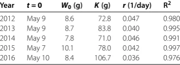
Table 1 summaries the identified parameters values andt= 0 in each year, which are used for drawing the figure.
Table 1 The initial timet= 0, the identifiedW0,K, andr, andR2value between the measured
and identifiedWtin each year
Year t = 0 W0(g) K(g) r(1/day) R2
2012 May 9 8.6 72.8 0.047 0.980
2013 May 9 8.7 83.8 0.040 0.995
2014 May 9 7.8 71.0 0.046 0.991
2015 May 7 10.1 78.0 0.042 0.997
2016 May 10 8.4 106.7 0.036 0.976
Figure shows the measured and fittedWtin each growth period from to . The
circles are measured values and the curves are fitted growth curves based on the Verhulst model.
Table summarizes the initial timet= . The table also shows the identified values of the parametersW,K, andrfor each year using a nonlinear least squares method with the Rvalue between the measured and identifiedWt. The order of the parametersW, K, andrare same in each year, while their values are slightly different between different years. Figure and Table show that the growth of aquaculturedP. altivelisin each year is accurately approximated with the conventional Verhulst model (). The identified result suggestsK=O() (g),W
=O() (g), andrT=O() (-); the last one follows from the discussion below. In what follows the data in is used in the numerical computation as a demonstrative application of the present model.
The terminal time is set asT= (day) considering current management strategy by HRFC. The optimal opening timeτ∗ is computed directly from () using the classical Simpson’s rule. The time increment for integrationτis set as . (day). The total num-ber of individuals at the timet= is specified asN= , based on an actual manage-ment strategy by HRFC. ThisNhas been empirically determined by HRFC considering the size of the pool used for their aquaculture.
The varianceVar[Nt], which is an index used for verifying optimal management strategy,
is obtained with the formula () in Appendix as
Var[Nt] =Var[Mt–τ] withk= ()
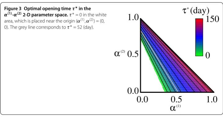
Figure 3 Optimal opening timeτ∗in the
α(1)-α(2)2-D parameter space.τ∗= 0 in the white
area, which is placed near the origin (α(1),α(2)) = (0,
0). The grey line corresponds toτ∗= 52 (day).
σ(n), while it is decreasing with respect to eacha(n). Comparing the magnitude of the three terms ofVar[Nt] (right-hand side of the formula () in Appendix ) can quantify and
qual-ify uncertainties involved in the management strategy.
Based on the personal communications with the officers of HRFC and their account-ing book duraccount-ing , the parametersλ(n)andC(n)are set asλ()= (/day),λ()= . (/day),C()= (kg),C()= , (kg), respectively. The parametersa(n)andσ(n)are set asa()=a()= (/day),σ()= (/day), andσ()= (/day). The parameterpis set as . (/day). The mortality rateRis set as . (/day) considering the fact that almost % of aquaculturedP. altivelisdied during the growth period in . There are three weight parametersα(),α(), andβin the model. Considering the form of the performance indexJτ, the following relationship is assumed without the loss of generality of analysis:
α()+α()+β= withα(),α(),β> . ()
Therefore, choosingα()andα()givesβasβ= – (α()+α()).
4.3 Computational results
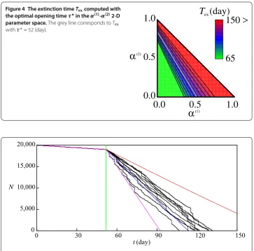
Figure plots the optimal opening timeτ∗in the -Dα()-α()parameter space. The grey line in the figure corresponds toτ∗by HRFC in . In addition, Figure plots the extinc-tion timeTexcomputed with the optimal opening timeτ∗in the -Dα()-α()parameter space. The grey line in the figure corresponds toTexby HRFC in . Figure shows consistency between the computational result and the mathematical analysis result since there exists an area withτ∗= near the origin (α(),α()) = (, ), at whichηis large and the inequality () is not satisfied. Figure also shows that the computational results are con-sistent with the Theorem .. The computational result suggests unique existence ofτ∗.
Conjecture . τ∗∈[,T]exists uniquely.
Figure plots E[Nt], E[Nt]±
√
Var[Nt], and ten sample paths ofNtassuming the actual
valueτ∗= (day) of HRFC in with the time increment for temporal integration . (day). The Runge-Kutta scheme [] has been used for generating the sample paths where
the transformation of variablesft=
Figure 4 The extinction timeTexcomputed with
the optimal opening timeτ∗in theα(1)-α(2)2-D
parameter space.The grey line corresponds toTex
withτ∗= 52 (day).
Figure 5 E[Nt] (blue),E[Nt] +√Var[Nt] (red),E[Nt] –√Var[Nt] (pink), and sample paths ofNt(black) assumingτ∗= 52 (green).Ten sample paths have been simulated using the strong numerical scheme (Wilkie [42]) with the time increment for temporal integration 0.01 (day).
additive noise term
dft=
ft
a(n)C(n)–(σ (n))
–a(n)ft
dt+σ (n) dB
(n)
t , t> , ()
which is easier to numerically handle []. The sample paths of Figure well characterize the behavior of Nt that it is monotonically decreasing due to frequent small shocks by
harvesting for sale and large and rare shocks for harvesting for ecological education, which is in accordance with the actual situation of HRFC. In the actual management strategy of P. altivelisby HRFC,Texin was (day). The modelled extinction timeTex with
τ∗ = (day) is . (day), which agrees well with the actual value by HRFC in ,
implying that the utilized parameter values are reasonable.
Finally, to compare impacts of the two different stochastic harvestings, the following stochastic variables that quantify the profit of the harvestings
j(n)=
T∧Tex(τ∗)
τ∗
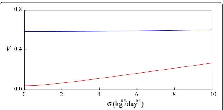
Figure 6 Numerically computedV(n)for 0≤σ(1),σ(2)≤10 (kg1/2/day1/2) withτ∗= 52 (day):n= 1
(harvesting for sale, red) andn= 2 (harvesting for ecological education, blue).
are considered. The non-dimensional indexes to evaluate relative variability of the profits are presented as
V(n)=
Var[j(n)]
E[j(n)] (n= , ), ()
which are computed with a numerical integration technique based on the standard mid-point rules. The indexV(n)measures the fluctuation of the processj(n)
τ relative to its mean
value. Therefore, largerV(n) implies relatively larger stochastic fluctuations ofj(n). The indexesV(n)are computed for different values ofσ(n)to evaluate dependence of the profits by harvestings for sale and ecological education on the stochasticity of demands.
Figure plots the numerically computedV(n) for ≤σ(),σ()≤ (kg//day/). Fig-ure shows that the indexes V(n) are larger in the harvesting for ecological education (n= ) than in the harvesting for sale (n= ). In addition, eachV(n) is monotonically in-creasing with respect toσ(n), and variability ofV(n)for the range ofσ(n)examined are larger in the harvesting for selling than in that for ecological education. The computational re-sults show that the harvesting for sale is more robust against the stochastic fluctuation of the demand, implying that it can be a major source of profit of the FC. Nevertheless, the harvesting for ecological education, although it turned out to be less robust with larger V(n), actually should not be abandoned since it has served as an indispensable part of the work of the FC. The computational results in this paper provide useful information for decision-making on management of aquaculture systems subject to the stochasticity.
5 Conclusion
where the harvesting for ecological education can be more efficiently carried out with wider spillover effects. Financial and social supports from local governments would be helpful for FCs to achieve this attempt.
Future research will develop an optimization theory for long-term, multi-year manage-ment of aquaculturedP. altivelis, so that FCs in Japan can find the way to achieve cost-effective management strategy of the fish. In addition, local economic dynamics around the FCs will also be mathematically described, so that the demand of the fishes is more reasonably tracked. Investigations both from theoretical and practical viewpoints are nec-essary for further advance of fishery science and engineering.
Appendix 1
This appendix presents a calculation procedure of the variance ofMt, which is defined
asVar[Mt] = E[Mt] – (E[Mt]). By the martingale property of the compensated Poisson
processP(tn)–λ(n)t(Chapter of []) and stationarity ofc
(n)
t , E[Mt] satisfies
exp(Rt)EMt
= E
M–
t
exp(Rs)
k
n=
c(sn)dPs(n)
=M– MB
exp(Rt) – + E
t
exp(Rs)
k
n=
λ(n)c(sn)ds
+ E
k
n=
λ(n)
t
c(n)
s
exp(Rs) ds
. ()
By stationarity and independency ofc(tn), the second term in the right-hand side of () becomes
E
t
exp(Rs)
k
n=
λ(n)c(sn)ds
= k m= k n=
λ(n)λ(m)
t
t
expR(s+u)Ec(m)
u c(sn)
dsdu
=
k
m=n,m≥,n≥
λ(m)λ(n)C(n)C(m)
exp(Rt) – R + k n=
λ(n)
t
t
expR(s+u)Ecu(n)c(sn)dsdu. ()
Then, () is rewritten as
exp(Rt)EMt=exp(Rt)E[Mt]
–Bexp(Rt) –
+
k
m=n,m≥,n≥
λ(m)λ(n)C(n)C(m)
exp(Rt) – R
+
k
n=
λ(n)
t
t
expR(s+u)Ecu(n)c(sn)dsdu
+ E
k
n=
λ(n)
t
c(sn)exp(Rs) ds
. () Note that E k n= t
c(sn)exp(Rs) ds
=(exp(Rt) – )(exp(Rt) + ) R
k
n=
C(n)(σ(n))
a(n) , () Ec(un)c(sn)=C
(n)(σ(n)) a(n) exp
–a(n)|u–s|+C(n), ()
k
n=
λ(n)
t
t
expR(s+u– t)Ecu(n)c(sn)dsdu
=B –exp(–Rt)
+
k
n=
(λ(n))C(n)(σ(n)) a(n)
t
t
expR(s+u– t) –a(n)|u–s|dsdu, ()
and
t
t
expR(s+u– t) –a(n)|u–s|dsdu
=exp(–Rt) R+a(n)
⎧ ⎨ ⎩
exp(Rt)–
R –t (R=a(n)),
exp(Rt)– R –
exp((R–a(n))t)–
R–a(n) (R=a(n)).
()
Therefore, with () through (), a closed-form expression of the varianceVar[Mt] is
obtained as
Var[Mt] = k
m=n,m≥,n≥
λ(m)λ(n)C(n)C(m)
–exp(–Rt) R + k n=
(λ(n))C(n)(σ(n)) a(n)
×
t
t
expR(s+u– t) –a(n)|u–s|dsdu
+( +exp(–Rt))( –exp(–Rt)) R
k
n=
λ(n)C(n)(σ(n))
a(n) . ()
The formula () shows thatVar[Mt] is increasing with respect to eachλ(n),C(n), andσ(n),
while it is decreasing with respect to eacha(n).
Appendix 2
This appendix shows calculation procedures of the first-order derivative ofJτ. A key of the
T>Tex, differentiating both-hand sides of () with respect toτ yields
dJτ
dτ =
d dτ ˜ A T τ
Wtds–βp
T
E[Nt]Wtdt
= –AW˜ τ–βpNexp(–Rτ)Wτ–βp
d dτ
T
τ
E[Nt]Wtdt. ()
Since
–βp d dτ
T
τ
E[Nt]Wtdt
=βp
Nexp(–Rτ)Wτ–BR
T
τ
exp–R(t–τ)Wtdt
, ()
combining () and () yields
dJτ
dτ = –AW˜ τ–βpBR
T
τ
exp–R(t–τ)Wtdt, ()
which is (). Similarly, forT>Tex,
dJτ
dτ =
d dτ ˜ A Tex τ
Wtds–βp
Tex
E[Nt]Wtdt
. ()
The first term in the right-hand side of () is calculated as
˜
A d dτ
Tex
τ
Wtds=A˜
dTex
dτ WTex–Wτ
=AF˜ τ. ()
By (), the second term in the right-hand side of () is calculated as
d dτ
–βp
Tex
E[Nt]Wtdt
= –βpd dτ
τ
E[Nt]Wtdt+
Tex
τ
E[Nt]Wtdt
= –βp
E[Nτ]Wτ+
dTex
dτ E[NTex]WTex
–Nexp(–Rτ)Wτ+
Tex
τ
d
dτE[Nt]Wtdt
= –A˜ηGτ ()
since E[NTex] = . Combining (), (), and () yields ().
Appendix 3
The following proposition used in Proposition . is proven in this appendix.
Proposition A. Assume p= and g is given by the generalized Verhulst model()with r>R andθ≥.In addition,assumeτ∗∈(,τex)solvesddJττ = .Then,
dJτ
Proof Under the stated assumption,dJτ
dτ atτ=τ∗is
˜
A dJ
τ
dτ =
dTex dτ
g(WTex)WTex+ dT
ex
dτ WTex–g(Wτ)Wτ, ()
which can be rewritten with () as
˜
A dJ
τ
dτ = Wτ
WTex
R–g(Wτ)
WTex+
g(WTex) –R
Wτ
atτ=τ∗. ()
Substituting () into () yields
˜
A dJτ
dτ = Wτ
WTex
–(r–R)(WTex–Wτ) –rK–θWτWTex
WTθ–ex –Wτθ–
< atτ=τ∗, ()
which withA˜ > proves the proposition.
Acknowledgements
The River Fund No. 285311020 in charges of The River Foundation, JSPS Research Grant Nos. 15H06417, 17K15345, and WEC Applied Ecology Research Grant No. 2016-02 support this research. The authors thank to Hii River Fishery Cooperatives for providing valuable data.
Funding
The River Fund No. 285311020 in charges of The River Foundation, JSPS Research Grant Nos. 15H06417, 17K15345, and WEC Applied Ecology Research Grant No. 2016-02 support this research.
Competing interests
The authors declare that they have no competing interests.
Authors’ contributions
HY wrote the paper with the support of YY. HY and YY performed mathematical and numerical analysis, and interviews to officers of Hii River Fisheries Cooperatives. All authors read and approved the final manuscript.
Authors’ information
Yuta Yaegashi is Research Fellow of Japan Society for the Promotion of Science.
Author details
1Faculty of Life and Environmental Science, Shimane University, Nishikawatsu-cho 1060, Matsue, Shimane 690-8504, Japan.2Graduate School of Agriculture, Kyoto University, Kitashirakawa-oiwake-cho, Sakyo-ku, Kyoto, Kyoto 606-8502, Japan.
Publisher’s Note
Springer Nature remains neutral with regard to jurisdictional claims in published maps and institutional affiliations.
Received: 13 March 2017 Accepted: 11 May 2017 References
1. Gjedrem T, Robinson N, Rye M. The importance of selective breeding in aquaculture to meet future demands for animal protein: a review. Aquaculture. 2012;350:117-29. doi:10.1016/j.aquaculture.2012.04.008.
2. Clarke JL, Waheed MT, Lössl AG, Martinussen I, Daniell H. How can plant genetic engineering contribute to cost-effective fish vaccine development for promoting sustainable aquaculture? Plant Mol Biol. 2013;83:33-40. doi:10.1007/s11103-013-0081-9.
3. Mazid MA, Zaher M, Begum NN, Ali MZ, Nahar F. Formulation of cost-effective feeds from locally available ingredients for carp polyculture system for increased production. Aquaculture. 1997;151:71-8.
doi:10.1016/S0044-8486(96)01504-9.
4. Myers RA, Barrowman NJ, Hutchings JA, Rosenberg AA. Population dynamics of exploited fish stocks at low population levels. Science. 1995;269(5227):1106. doi:10.1126/science.269.5227.1106.
5. Victor BC. Recruitment and population dynamics of a coral reef fish. Science. 1983;219(4583):419-20. doi:10.1126/science.219.4583.419.
7. Frigessi A, Holden L, Teigland A. (sfi)2statistics for innovation - the experience of the Oslo centre in industrial statistics. Appl Stoch Models Bus Ind. 2015;31:82-93. doi:10.1002/asmb.2113.
8. Llorente I, Luna L. Bioeconomic modelling in aquaculture: an overview of the literature. Aquac Int. 2015;24:1-18. doi:10.1007/s10499-015-9962-z.
9. McCausland WD, Mente E, Pierce GJ, Theodossiou I. A simulation model of sustainability of coastal communities: aquaculture, fishing, environment and labour markets. Ecol Model. 2006;193:271-94.
doi:10.1016/j.ecolmodel.2005.08.028.
10. Sana SS. Optimal pricing strategy for livestock of fishery and poultry. Econ Model. 2012;29:1024-34. doi:10.1016/j.econmod.2012.03.010.
11. Schechtman E, Wax Y, Tandler A. The effect of photoperiod and prey density on long-term survival of larvae - a data analytic approach where no parametric model is assumed and individual follow-up is not available. Appl Stoch Models Data Anal. 1990;6:27-40. doi:10.1002/asm.3150060104.
12. Øksendal B. Stochastic differential equations. Berlin: Springer; 2003.
13. Nøstbakken L. Regime switching in a fishery with stochastic stock and price. J Environ Econ Manag. 2006;51:231-41. doi:10.1016/j.jeem.2005.07.001.
14. Reed WJ, Clarke HR. Harvest decisions and asset valuation for biological resources exhibiting size-dependent stochastic growth. Int Econ Rev. 1990;31:147-69. doi:10.2307/2526634.
15. León-Santana M, Hernández JM. Optimum management and environmental protection in the aquaculture industry. Ecol Econ. 2008;64:849-57. doi:10.1016/j.ecolecon.2007.05.006.
16. Grantham RW, Rudd MA. Current status and future needs of economics research of inland fisheries. Fisheries Manag Ecol. 2015;22:458-71. doi:10.1111/fme.12144.
17. Welcomme RL, Cowx IG, Coates D, Béné C, Funge-Smith S, Halls A, Lorenzen K. Inland capture fisheries. Philos Trans R Soc Lond B, Biol Sci. 2010;365:2881-96. doi:10.1098/rstb.2010.0168.
18. Yoshioka H, Yaegashi Y. Finding the optimal opening time of harvesting farmed fishery resources. Pac J Math Ind. 2016;8:6. doi:10.1186/s40736-016-0025-9.
19. Yoshioka H, Yaegashi Y. Optimal criteria to start harvesting in stochastic aquaculture system. Appl Stoch Models Bus Ind. In press 2017. doi:10.1002/asmb.2250.
20. Dixit AK, Pindyck RS. Investment under uncertainty. Princeton: Princeton University Press; 1994.
21. Abe S, Sajiki T, Tamaki Y, Awata S, Iguchi K. Educational significance of fishermen’s activities providing opportunities for schoolchildren to play in streams. Jpn J Limnol (Rikusuigaku Zasshi). 2013;74:165-71. doi:10.3739/rikusui.74.165 (in Japanese with English abstract).
22. Oshitani M, Seki I, Hayashi H, Nishizaki T. The actual state of exchange between urban resident and fishing community and a subject of vitalization of region. Proc Civ Eng Ocean. 2004;20:311-5 (in Japanese with English abstract).
23. Japan Fisheries Agency. http://www.jfa.maff.go.jp/j/enoki/naisuimeninfo.html (2017). Accessed 1 Jan 2017. 24. Hii River Fisheries Cooperative. Se-oto (Annual public relations magazine published by HRFC), p. 5.
http://www.hiikawafish.jp/date/160701_seoto_no9.pdf. Accessed 28 Dec 2016.
25. Blanchard EA, Loxton R, Rehbock V. A computational algorithm for a class of non-smooth optimal control problems arising in aquaculture operations. Appl Math Comput. 2013;219:8738-46. doi:10.1016/j.amc.2013.02.070.
26. Neubert MG. Marine reserves and optimal harvesting. Ecol Lett. 2003;6:843-9. doi:10.1046/j.1461-0248.2003.00493.x. 27. Pascoe S, Wattage P, Naik D. Optimal harvesting strategies: practice versus theory. Aquac Econ Manag.
2002;6:295-308. doi:10.1080/13657300209380320.
28. Privault N. Notes on Stochastic Finance. https://drive.google.com/file/d/0B29QNyowSj9sM210Z2RaMG41VFE/edit (2014). Accessed 28 Dec 2016.
29. Ross SM. Applied probability models with optimization applications. New York: Dover; 2013. 30. Thieme HR. Mathematics in population biology. Princeton: Princeton University Press; 2003.
31. Strzałka D, Grabowski F. Towards possibleq-generalizations of the Malthus and Verhulst growth models. Phys A, Stat Mech Appl. 2008;387:2511-8. doi:10.1016/j.physa.2007.12.014.
32. Cox JC, Ingersoll JE, Ross SA. Theory of the term structure of interest rates. Econometrica. 1985;53:385-407. doi:10.2307/1911242.
33. Platen E, Bruti-Liberati N. Numerical solution of stochastic differential equations with jumps in finance. Heidelberg: Springer; 2010. p. 62.
34. Bensoussan A, Brouste A. Cox-Ingersoll-Ross model for wind speed modeling and forecasting. Wind Energy. 2015;19:1355-65. doi:10.1002/we.1896.
35. Campillo F, Joannides M, Larramendy-Valverde I. Stochastic modeling of the chemostat. Ecol Model. 2011;222:2676-89. doi:10.1016/j.ecolmodel.2011.04.027.
36. MAFF. Statistics agriculture, forestry and fisheries in Japan during 2014 (in Japanese).
http://www.maff.go.jp/j/tokei/kouhyou/kaimen_gyosei/pdf/gyogyou_seisan_14.pdf. Accessed 25 Jun 2016. 37. Katano O, Abe S, Nakamura T. Relationships between ayuPlecoglossus altivelis altivelisand other organisms in stream
communities. Bull Fish Res Agency. 2006;Suppl 5:203-8 (in Japanese with English abstract).
38. Takahashi I, Azuma K. The up-to-now knowledge book of ayu. Tokyo: Tsukiji-shokan; 2006 (in Japanese). 39. Tanaka Y, Iguchi K, Yoshimura J, Nakagiri N, Tainaka K. Historical effect in the territoriality of ayu fish. J Theor Biol.
2011;268:98-104. doi:10.1016/j.jtbi.2010.09.040.
40. Tago Y. Survival of a landlocked form of ayu fry released in the Shou River. Aquac Sci. 1999;47:111-2. doi:10.11233/aquaculturesci1953.47.111 (in Japanese).
41. Kumada N, Arima T, Tsuboi JI, Ashizawa A, Fujioka M. The multi-scale aggregative response of cormorants to the mass stocking of fish in rivers. Fish Res. 2013;137:81-7. doi:10.1016/j.fishres.2012.09.005.
42. Wilkie J. Numerical methods for stochastic differential equations. Phys Rev E. 2004;70:017701. doi:10.1103/PhysRevE.70.017701.