1
Bayesian Cognitive Science, Unification, and Explanation
Matteo Colombo and Stephan Hartmann
Abstract
It is often claimed that the greatest value of the Bayesian framework in cognitive science consists in its unifying power. Several Bayesian cognitive scientists assume that unification is obviously linked to explanatory power. But this link is not obvious, as unification in science is a heterogeneous notion, which may have little to do with explanation. While a crucial feature of most adequate explanations in cognitive science is that they reveal aspects of the causal mechanism that produces the phenomenon to be explained, the kind of unification afforded by the Bayesian framework to cognitive science does not necessarily reveal aspects of a mechanism. Bayesian unification, nonetheless, can place fruitful constraints on causal-mechanical explanation.
Keywords Bayesian modelling; Unification; Causal-mechanical explanation; Cue integration; Computational cognitive neuroscience
1 Introduction
2 What a great many phenomena Bayesian decision theory can model
3 The Case of information integration
4 How do Bayesian models unify?
5 Bayesian Unification. What constraints on mechanistic explanation?
5.1Unification constrains mechanism discovery
5.2 Unification constrains the identification of relevant mechanistic factors
5.3 Unification constrains confirmation of competitive mechanistic models
6 Conclusion
2
1 Introduction
A recurrent claim made in the growing literature in Bayesian cognitive science is that one of the greatest values of studying phenomena such as perception, action, categorization, reasoning, learning, and decision-making within the framework of Bayesian decision theory1 consists in the unifying power of this modelling framework. Josh Tenenbaum and colleagues, for example, emphasise that Bayesian decision theory provides us with a ‘unifying mathematical language for framing cognition as the solution to inductive problems’ (Tenenbaum et al. [2011], p. 1285).
An assumption often implicit in this literature is that unification obviously bears on explanation. Griffiths et al. ([2010], p. 360), for example, claim that ‘probabilistic models provide a unifying framework for explaining the inferences that people make in different settings.’ Clark ([2013], p. 201) writes that ‘one way to think about the primary ‘added value’ of these [kinds of Bayesian] models is that they bring perception, action, and attention into a single unifying framework. They thus constitute the perfect explanatory partner… for recent approaches that stress the embodied, environmentally embedded, dimensions of mind and reason’ (emphasis added). Even more explicit is Friston ([2009], [2010]). He suggests that the unification afforded to cognitive science by the Bayesian framework might be driven by a specific hypothesis, which he calls the “free-energy principle,” concerning how different phenomena are brought about by a single type of
mechanism. Friston writes: ‘If one looks at the brain as implementing this scheme (minimising a variational bound on disorder), nearly every aspect of its anatomy and physiology starts to make sense’ (Friston [2009], p. 293); ‘a recently proposed free-energy principle for adaptive systems tries to provide a unified account of action, perception and learning... the principle [can] account for many aspects of brain structure and function and lends it the potential to unify different perspectives on how the brain works’ (Friston [2010], p. 127). Along the same lines, Hohwy ([2013], p. 1)
1
3 claims that the idea that brains are kinds of Bayesian machines constantly attempting to minimizing prediction errors ‘has enormous unifying power and yet it can explain in detail too.’
However, the link between unification and explanation is far from obvious (Morrison, [2000]). It is not clear in which sense the kind of unification produced by Bayesian modelling in cognitive science is explanatory. If the relationship between unification, explanation, and Bayesian modelling in cognitive science is elucidated, then the debate over the virtues and pitfalls of the Bayesian approach (Bowers and Davis [2012a], [2012b]; Jones and Love [2011]; for a reply see Griffiths et al. [2012]) will make a step forward.
4 interest, then Bayesian unification has genuine explanatory traction. Our novel contribution to existing literature is summarised in the conclusion.
2 What a great many phenomena Bayesian decision theory can model
Statistical inference is the process of drawing conclusions about an unknown distribution from data generated by that distribution. Bayesian inference is a type of statistical inference where data (evidence, or new information) are used to update the probability that a hypothesis is true. Probabilities are used to represent degrees of belief in different hypotheses (or propositions). At the core of Bayesian inference and Bayesian epistemology, there is a rule of conditionalization, which prescribes how to revise degrees of belief in different hypotheses in response to new data.
Consider an agent who is trying to infer the process that generated some data, d. Let H be a set of (exhaustive and mutually exclusive) hypotheses about this process (known as ‘hypothesis space’). For each hypothesis h H, P(h) is the probability that the agent assigns to h being the true
generating process, prior to observing the data d. P(h) is known as the ‘prior’ probability. The Bayesian rule of conditionalization prescribes that, after observing data d, the agent should update P(h) by replacing it with P(h | d) (known as the ‘posterior probability’). To execute the rule of conditionalization, the agent multiplies the prior P(h) by the likelihood P(d | h) as stated by Bayes’ theorem:2
[1] 𝑃(ℎ|𝑑) = ∑ 𝑃(𝑑|ℎ)𝑃(ℎ)𝑃(𝑑|ℎ)𝑃(ℎ)
ℎ∈𝐻
where P(d | h) is the probability of observing d if h were true (known as ‘likelihood’), and the sum in the denominator ensures that the resulting probabilities sum to one. According to [1], the posterior probability of h is directly proportional to the product of its prior probability and likelihood, relative to the sum of the products and likelihoods for all alternative hypotheses in the
2
5 hypothesis space H. The rule of conditionalization prescribes that the agent should adopt the posterior P(h | d) as a revised probability assignment for h: the new probability of h should be proportional to its prior probability multiplied by its likelihood.
Bayesian conditionalization alone does not specify how an agent’s beliefs should be used to generate a decision or an action. How to use the posterior distribution to generate a decision is described by Bayesian decision theory, and requires the definition of a loss (or utility) function L(A,
H). For each action a A—where A is the space of possible actions or decisions available to the
agent—the loss function specifies the relative cost of taking action a for each possible h H. To
choose the best action, the agent calculates the expected loss for each a, which is the loss averaged across the possible h, weighted by the degree of belief in h. The action with the minimum expected loss is the best action that the agent can take given her beliefs.
Cognitive scientists have been increasingly using Bayesian decision theory as a modelling framework to address questions about many different phenomena. As a framework, Bayesian decision theory is comprised of a set of theoretical principles, and tools grounded in Bayesian belief updating. Bayesian models are particular mathematical equations that are derived from such principles. Despite several important differences, all Bayesian models share a common, core structure. They capture a process that is assumed to generate some observed data, by specifying: 1) the hypothesis space under consideration, 2) the prior probability of each hypothesis in the hypothesis space, and 3) the relationship between hypotheses and data. The prior of each hypothesis is updated in light of new data according to Bayesian conditionalization, which yields new probabilities for each hypothesis. Bayesian models allow us to evaluate different hypotheses about some generative process, and to make inferences based on this evaluation.
6 learning, for example, can be modelled as the problem of learning the causal structure, associated to a certain probability distribution, responsible for generating some observed events; categorization can be framed as the problem of learning the distribution responsible for generating the exemplars of a category; perception can be understood as the problem of inferring the state of the world that produced current sensory input. So, most Bayesian models of cognition are hypotheses formulated in probabilistic terms about the type of computational problem that must be solved by an agent in order for the agent to display certain cognitive phenomena. As it will be clearer in the following sections, most Bayesian models are not hypotheses about the mechanisms that produce particular cognitive phenomena. They typically say nothing about the spatio-temporally organized components and causal activities that may produce particular cognitive phenomena, other than that such components and activities—whatever they are—must yield a solution with particular properties to a specific computational problem.3
Among the phenomena recently modelled within the Bayesian framework are4: categorization (Anderson [1991]; Kruschke [2006]; Sanborn et al. [2010]; see also Danks [2007]), causal reasoning (Pearl [2000]; Griffiths and Tenenbaum [2009]), judgement and decision-making (Beck et al. [2008]; Griffiths and Tenenbaum [2006]; see also Oaksford and Chater [2007]), reasoning about other agents’ beliefs and desires (Baker, Saxe, and Tenenbaum [2011]), perception
3
Marr’s ([1982]) three-level framework of analysis is often used to put into sharper focus the nature of Bayesian models of cognition (see Griffiths et al. [2010]; Colombo and Seriès [2012]; Griffiths et al. [2012]). Marr’s computational level specifies the problem to be solved in terms of some generic input-output mapping, and of some general principle by which the solution to the problem can be computed. In the case of Bayesian modelling, if the problem is one of extracting some property of a noisy stimulus, the general “principle” is Bayesian conditionalization and the generic input-output mapping that defines the computational problem is a function mapping the noisy sensory input to an estimate of the stimulus that caused that input. It is ‘generic’ in that it does not specify any
particular class of rules for generating the output. Such class is defined at the algorithmic level. The algorithm specifies how the problem can be solved. Many Bayesian models belong to this level, since they provide us with one class of methods for producing an estimate of a stimulus variable as a function of noisy and ambiguous sensory information. The level of implementation is the level of physical parts and their organization. It describes the biological mechanism that carries out the algorithm.
4
7 (Knill and Richards [1996]), illusions (Weiss, Simoncelli, and Adelson [2002]), psychosis (Fletcher and Frith [2009]), motor control (Körding and Wolpert [2004]; Wolpert and Landy [2012]), and language (Goldwater et al. [2009]; Perfors et al. [2011]; Xu and Tenenbaum [2007]).
This overview should be sufficient to give a sense of the breadth of the phenomena that can be modelled within the Bayesian framework. Given this breadth, a question worth asking is: How is unification actually produced within Bayesian cognitive science? To answer this question we turn to examine the case of cue integration. The reasons why we focus on this case are twofold. First, cue integration is one of the most studied phenomena within Bayesian cognitive science. In fact, cue integration ‘has become the poster child for Bayesian inference in the nervous system’ (Beierholm et al. [2008]). So, we take this case to be paradigmatic of the Bayesian approach. Second, sensory cue integration has been claimed to be ‘[p]erhaps the most persuasive evidence’ for the hypotheses that brains perform Bayesian inference and encode probability distributions (Knill and Pouget [2004], p. 713; see Colombo and Seriès [2012], for a critical evaluation of this claim). So, we believe that this case is particularly congenial to explore the question of which constraints Bayesian unification can place on causal-mechanical explanation in cognitive science, which will be the topic of Section 4.
3 The case of information integration
8 determined as a function of prior knowledge and the uncertainty associated with each piece of information. Let us make this idea precise.
Call S a random variable that takes on one of a set of possible values s1, …, sn of some
physical property. A physical property of an object is any measurable property of that object—e.g. length. The value s1 of S describes the state of that object with respect to that property at a moment
in time. Call M a sequence of measurements m1,…, mn of a physical property. M can be understood
as a sequence of ‘cues’ or signals, which can be obtained from different sources of information (or modalities). Call Mi and Mj two sequences of measurements obtained respectively through
modalities i and j. Measurements Mi and Mj can be corrupted by noise, which can cause particular
measurements mi and mj to yield the wrong value for a given s. Given two sequences of
measurements Mi and Mj of the property S, and assuming that their noises are independent,5 the
likelihood function P(Mi, Mj | S) can be derived, which describes how likely it is that any value of S
gives rise to measurements (Mi, Mj). If we assume that the prior P(S) is uniform6 (i.e. a constant)
and we know the mean and variance of the probability distributions associated with the sequences of measurements Mi and Mj in isolation, we can derive the mean and variance of the Bayes-optimal
bimodal estimate in the following way.
If σMi2 is the variance of the estimate of S based on measurements (‘cues’ or signals) from
the source i, and σMj2 is the variance of the estimate of S based on measurements from the source j,
and the likelihoods are Gaussian, that is:
5
Different modalities are independent when the conditional probability distribution of either, given the observed value of the other, is the same as if the other’s value had not been observed. In much work on cue integration, independence has generally been assumed. This assumption can be justified empirically by the fact that the cues come from different, largely separated sensory modalities—for example, by the fact that the neurons processing visual information are far apart from the cortical neurons processing haptic information in the cortex. If the cues are less clearly independent, such as e.g. texture and linear perspective as visual cues to depth, cue integration should take into account the covariance structure of the cues (see Oruç, Maloney, and Landy [2003]).
6
To say that the Bayesian prior is uniform is to say that all values of S are equally likely before any measurement Mi. This assumption can be justified by the fact that e.g. experimental participants
9 [2] 𝑃(𝑀𝑖|𝑆) ∝ exp (−(𝑀𝑖−𝑆)
2
2𝜎𝑀𝑖2 )
[2’] 𝑃(𝑀𝑗|𝑆) ∝ exp (−(𝑀𝑗−𝑆)2 2𝜎𝑀𝑗2 )
then the posterior distribution of S given Mi and Mj will also be a Gaussian. From Bayes’ theorem,
and [2] and [2’], it follows that:
[3] 𝑃(𝑆|𝑀𝑖, 𝑀𝑗) ∝ exp (−(𝑀𝑖−𝑆)
2
2𝜎𝑀𝑖2 −
(𝑀𝑗−𝑆)2
2𝜎𝑀𝑗2 ) ∝ exp(−
(𝑆−𝜎𝑀𝑖2 𝑀𝑗+𝜎𝑀2 𝑀𝑖𝑗 𝜎𝑀𝑖2 + 𝜎𝑀𝑗2 )
2
2 𝜎𝑀𝑖2 𝜎𝑀𝑗 2
𝜎𝑀𝑖2 + 𝜎𝑀𝑗2 )
The maximum of this distribution is also the mean of the following Gaussian:
[4] 〈𝑆〉 = 𝜎𝑀𝑖
2
𝜎𝑀𝑖2 + 𝜎𝑀𝑗2 𝑀𝑗+ 𝜎𝑀𝑗2
𝜎𝑀𝑖2 + 𝜎𝑀𝑗2 𝑀𝑖
This mean will fall between the mean estimates given by each isolated measurement (if they differ) and will tend to be pushed towards the most reliable measurement. Its variance is:
[5] 𝜎𝑆2 =
𝜎𝑀𝑖2 𝜎𝑀𝑗2
𝜎𝑀𝑖2 + 𝜎𝑀𝑗2
The combined reliability is then equal to the sum of individual sources reliabilities:
[6] 𝜎1
𝑆2 = 1 𝜎𝑀𝑖2 +
1 𝜎𝑀𝑗2
This entails that the reliability of the estimate of S based on the Bayesian integration of information from two different sources i and j will be always greater than that based on information from each individual source alone.
10 their reliability, as shown in equation [4]. This resulting integrated distribution will have minimal variance. Call this “linear model for maximum reliability.”
This type of model has been used to account for several phenomena, including sensory, motor, and social phenomena. Ernst and Banks ([2002]) considered the problem of integrating information about the size of a target object from vision and touch. They asked their experimental participants to judge which of two sequentially presented objects was the taller. Participants could make this judgement by relying on vision alone, touch alone, or vision and touch together. For each of these conditions, the proportion of trials in which the participant judged that the ‘comparison
stimulus object’ (with variable height) was taller than the ‘standard stimulus object’ (with fixed height) was plotted as a function of the height of the comparison stimulus. These psychometric functions represented the accuracy of participants’ judgements, and were well fit by cumulative
Gaussian functions, which provided the variances σV2 and σT2 for the two within-modality
distributions of judgements. It should be noted that various levels of noise were introduced in the visual stimuli to manipulate their reliability. From the within-modality data, and in accordance to equations [3], [4], and [5], Ernst and Banks could derive a Bayesian integrator of the visual and tactile measurements obtained experimentally. They assumed that the loss function of their participants was quadratic in error, that is L (S, f (Mi)) = (S - f (Mi))2, so that the predicted optimal
estimate based on both sources of information was the mean of the posterior (as per [4]). The predicted variance σVT2 of the visual-tactile estimates was found to be very similar to the one
11 Exactly the same types of experimental and modelling approaches were adopted by Knill and Saunders ([2003], p. 2539) to ‘test whether the human visual system integrates stereo and texture information to estimate surface slant in a statistically optimal way’, and by Alais and Burr ([2004]) to test how visual and auditory cues could be integrated to estimate spatial location. Their behavioural results were predicted by a Bayesian linear model of the type described above, where information from each available source is combined to produce a stimulus estimate with the lowest possible variance.
These results demonstrate that the same type of model could be used to account for perceptual phenomena such as multi-modal integration (Ernst and Banks [2002]), uni-modal integration (Knill and Saunders [2003]), and the ‘ventriloquist effect’—i.e. the perception of speech sounds as coming from a spatial location other than their true one (Alais and Burr [2004]).
Besides perceptual phenomena, the same type of model can be used to study sensorimotor phenomena. In Körding and Wolpert’s ([2004]) experiment, participants had to reach a visual target with their right index finger. Participants could never see their hands; on a projection-mirror system, they could see, instead, a blue circle representing the starting location of their finger, a green circle representing the target, and a cursor representing the finger’s position. As soon as they moved their finger from the starting position, the cursor disappeared, shifting laterally relative to the actual finger location. The hand was never visible. Midway during the reaching movement, visual feedback of the cursor centered at the displaced finger position was flashed, which provided information about the current lateral shift. On each trial, the lateral shift was randomly drawn from a Gaussian distribution, to which Körding and Wolpert referred as ‘true prior.’ The reliability of the
12 account how reliable the visual feedback was (i.e. the likelihood of perceiving a lateral shift xperceived
when the true lateral shift is xtrue), and combined these pieces of information in a Bayesian way,
then participants’ estimate of xtrue of the current trial given xperceived should have moved towards the
mean of the prior distribution P(xtrue) by an amount that depended on the reliability of the visual
feedback. For Gaussian distributions this estimate is captured by [4], and has the smallest mean squared error. It is a weighted sum of the mean of the ‘true prior’ and the perceived feedback position:
[4’] 〈𝑥〉 = 𝜎 𝜎𝑥𝑝𝑒𝑟𝑐𝑒𝑖𝑣𝑒𝑑2
𝑥𝑝𝑒𝑟𝑐𝑒𝑖𝑣𝑒𝑑2 + 𝜎𝑥𝑡𝑟𝑢𝑒2 𝜇𝑥𝑡𝑟𝑢𝑒+
𝜎𝑥𝑡𝑟𝑢𝑒2
𝜎𝑥𝑝𝑒𝑟𝑐𝑒𝑖𝑣𝑒𝑑2 + 𝜎𝑥𝑡𝑟𝑢𝑒2 𝑥𝑝𝑒𝑟𝑐𝑒𝑖𝑣𝑒𝑑
Körding and Wolpert found that participants’ performance matched the predictions made by [4’]. They concluded that participants ‘implicitly use Bayesian statistics’ during their sensorimotor task, and ‘such a Bayesian process might be fundamental to all aspects of sensorimotor control and learning’ (p. 246).
Let us conclude this section by turning to social decision-making. Sorkin et al. ([2001]) investigated how groups of people can combine information from their individual members to make an effective collective decision in a visual detection task. The visual detection task consisted in judging whether a visual stimulus presented in each experimental trial was drawn either from a “signal-plus-noise” or from a “noise-alone” distribution. Each participant had, firstly, to carry out
the task individually; after the individual sessions, participants were tested in groups, whose size varied between three and ten members.
A model conceptually identical to the one used in research in multi-sensory perception was adopted. Each individual member of the group corresponded to a source of information, whose noise was assumed to be Gaussian and independent of other sources’ noise. Individual group members’ decisions i in the task were based on their noisy perceptual estimates, which could be modelled as Gaussian distributions with mean i and standard deviation i. The collective decision
13 competence at the task—where competence is the inverse of the variance of individual’s decisions,
2
i. According to Sorkin and colleagues’ model of social decision-making, in reaching a collective
decision, individual group members i communicated a measure of confidence in their decisions. The measure communicated to the group corresponded to both i and i. Individual and group
psychometric functions were fit with a cumulative function, with bias b and variance 2. The slope si of this function provides an estimate of the reliability of the individual estimates (i.e. the
individual’s competence at the task) thus:
[7] 𝑠𝑖 = 1
√2𝜋𝜎𝑖2
A large si corresponds to small variance, and hence to highly reliable decisions. Now, for groups of
n members that have a specified mean, variance, and correlation, the group bias bgroup is given in
terms of the individual biases as:
[8] 𝑏𝑔𝑟𝑜𝑢𝑝 = ∑ 𝑠𝑖 2𝑏
𝑖 𝑛 𝑖=1 ∑𝑛𝑖=1𝑠𝑖2
And the group slope (i.e. group reliability) sgroup is given as:
[9] 𝑠𝑔𝑟𝑜𝑢𝑝 = √∑𝑛𝑖=1𝑠𝑖2
Equations [8] and [9] are derived from [4] above, as they specify that a statistically optimal way to integrate information during collective decision making is to form a weighted average of the different individual members’ judgements. This model was shown to accurately predict group
performance. Consistently with the model, group’s performance was generally better than individual performances. When individual decisions were collectively discussed, performance generally accrued over and above the performance of the individual members of the group. Inconsistently with the model’s predictions, performance tended to decrease as group size increased. This finding, however, was not attributed to inefficiency in combining the information provided by individual members’ judgements. Rather, Sorkin and colleagues explained it in terms
14 Bahrami et al. ([2010]) performed a similar study. They investigated pairs of participants making collective, perceptual decisions. Psychometric functions for individual participants and pairs were fit with a cumulative Gaussian function. They compared the psychometric functions derived from experimental data to the predictions made by four models, one of which was the linear model for maximum reliability. In line with Sorkin and colleagues’ ([2001]) results, and consistently with equations [8], and [9], pairs with similarly perceptually sensitive individuals (i.e. similarly reliable) were found to produce collective decisions that were close to optimal. Decisions of pairs of individuals with different sensitivities, however, were best predicted by a different model, according to which the type of information communicated between individuals i during
collective decision-making is the ratio i /i (i.e., a z-score of the distribution of their individual
decisions). The resulting model assumes that during collective decision-making there is a systematic failure in aggregating individual information such that decisions of the least reliable individual in the group are over-weighted. As the difference between two observers’ perceptual sensitivities increases, collective decisions are worse than the more sensitive individual’s decision. Hence, according to this model, collective decisions rarely outperform the individual decisions of their best members.
4 How do Bayesian models unify?
The kind of unification afforded by Bayesian models to cognitive phenomena does not reveal per se the causal structure of a mechanism. The unifying power of the Bayesian approach in cognitive science arises in virtue of the mathematics that it employs: this approach shows how a wide variety of phenomena obey regularities that are captured by few mathematical equations. Such equations do not purport to capture the causal structure underlying a given phenomenon. Bayesian modelling does not typically work by formulating an encompassing hypothesis about the world’s causal
15 mechanism that might be responsible for various phenomena. The case of information integration illustrates these two points well.
The fact that a common mathematical model of the type captured by equation [4] can be applied to a range of diverse phenomena, from sensory cue integration to instances of collective decision-making, does not warrant by itself that we have achieved a causal unification of these phenomena. The applicability of the model to certain phenomena, furthermore, is constrained by general mathematical results, rather than by evidence about how certain types of widespread regularities fit into the causal structure of the world. Let us substantiate these claims, in light of the basic idea underlying the unificationist account of explanation.
According to the unificationist account of explanation, explanation is a matter of unifying a range of diverse phenomena with a few argument patterns (Kitcher [1989]; see also Friedman [1974]). The basic idea is that ‘science advances our understanding of nature by showing us how to derive descriptions of many phenomena, using the same pattern of derivation again and again, and in demonstrating this, it teaches us how to reduce the number of facts that we have to accept as ultimate’ (Kitcher [1989], p. 423). Kitcher makes this idea precise by defining a number of
technical terms. For our purposes, it suffices to point to the general form of the pattern of derivation involved in our case study. Spelling out this pattern will make it clear how the applicability of a Bayesian model to certain phenomena is constrained by general mathematical results, rather than by evidence about how certain types of widespread regularities fit into the causal structure of the world.7
7
According to a unificationist, the applicability of a model to several phenomena need not be constrained by causal information for the model to be explanatory. In this paper, we remain
agnostic about whether a particular unificationist account of explanation fits explanatory practice in cognitive science, and about whether the type of unification afforded by Bayesian modelling to cognitive science fits Kitcher’s ([1989]) account of explanation. If Bayesian unification in cognitive science actually fits Kitcher’s ([1989]) account, then there would be grounds to support the
16 Let us consider a statement like: ‘The human cognitive system integrates visual and tactile information in a statistically optimal way.’ This statement can be associated with a mathematical, probabilistic representation that abstracts away from the concrete causal relationships that can be picked out by the statement. Following Pincock’s ([2012]) classification, we can call this type of mathematical representation abstract acausal. The mathematical representation specifies a function from a set of inputs (i.e. individual sources of information) to a set of outputs (i.e. the information resulting from integration of individual sources). The function captures what ‘to integrate visual and tactile information in a statistically optimal way’ could mean. In order to build such a
representation, we may define two random variables (on a set of possible outcomes, and probability distributions) respectively associated with visual and tactile information. If these variables have certain mathematical properties (i.e., they are normally distributed, and their noises are independent), then one possible mathematical representation of the statement corresponds to equation [4], which picks out a family of linear models (or functions) of information integration for maximal reliability.
According to this type of mathematical representation, two individual pieces of information are integrated by weighting each of the two in proportion to its reliability (i.e. the inverse variance of the associated probability distribution). The relationship between the individual pieces of information, and the integrated information captures what ‘statistically optimal information integration’ could mean, viz.: information is integrated based on a minimum-variance criterion. The
same type of relationship can hold not only for visual and tactile information, but for any piece of information associated with a random variable, whose distribution has certain mathematical properties. Drawing on this type of relationship, we can derive descriptions of a wide variety of phenomena, regardless of the details of the particular mechanism producing the phenomenon.
17 What allows the derivations of all these descriptions is the wide scope of applicability of the linear model for maximum reliability expressed in the language of probability. The scope of applicability of the model is constrained by mathematical results, rather than by evidence about some causal structure. This model is an instance of what Pincock’s ([2012]) dubs abstract varying mathematical representations: ‘With an abstract varying representation we can bring together a
collection of representations in virtue of the mathematics that they share, and it can turn out that the success of this family of representations is partly due to this mathematical similarity’ (Pincock
[2012], p. 6). So, what unites all the descriptions of phenomena derivable from the linear model for information integration is an underlying mathematical relation, furnished by an abstract, more general, mathematical framework, viz.: the Bayesian framework, which serves as unifying language that uses probability distributions and Bayesian conditionalization in order to represent uncertainty and update belief in a given hypothesis in light of new information.
Let us conclude this section by considering the claim that the applicability of a model such as the linear model for information integration to several phenomena does not warrant by itself that a causal unification of these phenomena is achieved. One way to substantiate it is by examining the types of conclusions made by the studies surveyed in the section above about the mechanism underlying the phenomenon of interest. Ernst and Banks ([2002]) suggest that the neural mechanism of sensory cue-integration need not explicitly calculate the variances (and therefore the weights) associated with visual and tactile estimators for each property and situation. A neural mechanism for Bayesian cue integration—Ernst and Banks surmise—might compute an estimate of those variances ‘through interactions among populations of visual and haptic [i.e. tactile] neurons’ by
18 261) acknowledge that they ‘can only guess at the mechanism involved.’ Körding and Wolpert ([2004], p. 244) claim that ‘the central nervous system… employs probabilistic models during sensorimotor learning.’ However, this claim is left unarticulated. It is only noted that ‘a Bayesian view of sensorimotor learning is consistent with neurophysiological studies showing that the brain represents the degree of uncertainty when estimating rewards’ (p. 246). Sorkin et al. ([2001]) as
well as Bahrami et al. ([2010]) focused on how group performance depended on the reliability of the members, the group size, the correlation among members’ judgments, and the constraints on
member interaction. The conclusions that they drew from the application of Bayesian models to group decisions in their experiments did not include any suggestion, or any hypothesis, about the mechanism underlying group performance. Finally, Knill and Saunders ([2003]) explicitly profess agnosticism about the mechanism underlying their participants (Bayesian) performance. They make it clear right at the beginning that they considered ‘the system for estimating surface slant to be a black box with inputs coming from stereo and texture and an output giving some representation of surface orientation’ (p. 2541). Even if a linear model for cue integration successfully matched their participants’ performance, they explain: ‘psychophysical measurements of cue weights do not, in
themselves, tell us much about mechanism. More importantly, we believe that interpreting the linear model as a direct reflection of computational structures built into visual processing is somewhat implausible’ (p. 2556).
19 In sum, unification in Bayesian cognitive science is most plausibly understood as the product of the mathematics of Bayesian decision theory, rather than of a causal hypothesis concerning how different phenomena are brought about by a single kind of mechanism. If models in cognitive science ‘carry explanatory force to the extent, and only to the extent, that they reveal
(however dimly) aspects of the causal structure of a mechanism’ (Kaplan and Craver [2011], p. 602), then Bayesian models, and Bayesian unification in cognitive science more generally, do not have explanatory force. Rather than addressing the issue of under which conditions a model is explanatory, we accept that a crucial feature of many adequate explanations in the cognitive sciences is that they reveal aspects of the causal structure of the mechanism that produces the phenomenon to be explained. In light of this plausible claim, we ask what we consider a more fruitful question: What sorts of constraints can Bayesian unification place on causal-mechanical explanation in cognitive science? If these constraints contribute to revealing some relevant aspects of the mechanisms that produce phenomena of interest, then Bayesian unification has genuine explanatory traction.
5 Bayesian unification. What constraints on mechanistic explanation?
There are at least three types of defeasible constraints that Bayesian unification8 can place on causal-mechanical explanation in cognitive science. The first type of constraint is on mechanism discovery; the second type is on the identification of factors that can be relevant to mechanisms’ phenomena; the last type of constraint is on confirmation and selection of competing mechanistic models.
5.1 Unification constrains mechanism discovery
Several philosophers have explored the question of how mechanisms are discovered (Bechtel [2006]; Bechtel and Richardson [1993]; Craver and Darden [2001]; Darden and Craver [2002];
8
20 Darden [2006]; Thagard [2003]). If mechanisms consist of spatio-temporally organized components and causal activities, then, in order to discover mechanisms, we need strategies to identify components, their activities, and how they are spatio-temporally organized. One heuristic approach motivated by Bayesian unification constrains the search space for mechanisms. The strategy of this approach is as follows: If behaviour in a variety of different tasks is well-predicted by a given model, then presume that some features of the model map onto some common features of the neural mechanisms underlying that behaviour.
According to this strategy, the success of a Bayesian model in unifying several behavioural phenomena grounds the presumption that the underlying neural mechanisms possess features that correspond to features of the Bayesian model. Put differently, the success of a given Bayesian model in unifying several behavioural phenomena provides grounds for presuming that there is an isomorphism between the behavioural (or psychophysical) model and the model of the underlying neural mechanism.9
This heuristic approach to mechanism discovery is widespread in areas of cognitive science such as computational cognitive neuroscience, where a growing number of theoretical as well as empirical studies have started to explore how neural mechanisms could implement the types of Bayesian models that unify phenomena displayed in many psychophysical tasks (Rao [2004]; Ma et al. [2008]; Beck et al. [2008]; Deneve [2008]). The basic idea is to establish a mapping between psychophysics and neurophysiology that could serve as a starting point to investigate how activity in specific populations of neurons can account for the behaviour observed in certain tasks. Typically, the mapping is established by using two different parameterizations of the same type of Bayesian model.
9
21 For example, the linear model used to account for a wide range of phenomena in psychophysical tasks includes perceptual weights on different sources of perceptual information that are proportional to the reliability of such sources. If we presume that there is an isomorphism (or similarity relation) between this model and a model of the underlying neural mechanism, then neurons of this underlying mechanism should combine their inputs linearly with neural weights proportional to the reliability of the inputs. While the behavioural model includes Gaussian random variables corresponding to different perceptual cues and parameters corresponding to weights on each perceptual cue, the neural model includes different neural tuning curves10 and parameters corresponding to weights on each tuning curve. Drawing on this mapping, one prediction is that neural and perceptual weights will exhibit the same type of dependence on cue reliability. This can be determined experimentally, and would provide information relevant to discover neural mechanisms mediating a widespread type of statistical inference.
More concretely, Fetsch et al. ([2011]) provide an illustration of how Bayesian unification can constrain the search space for mechanisms, demonstrating one way in which a mapping can be established between psychophysics and neurophysiology. This study asked how multisensory neurons combine their inputs to produce behavioural and perceptual phenomena that require integration of multiple sources of information. To answer this question, Fetsch and colleagues trained macaque monkeys to perform a heading discrimination task, where the monkeys had to make estimations of their heading direction (i.e., to the right or to the left) based on a combination of vestibular and visual motion cues with varying degree of noise. Single-neuron activity was recorded from the monkeys’ dorsal medial superior temporal area (MSTd), which is a brain area that receives both visual and vestibular neural signals related to self-motion.
Fetsch and colleagues used a standard linear model of information integration, where heading signal was the weighted sum of vestibular and visual heading signals, and the weight of
10
22 each signal was proportional to its reliability. This model was used to account for the monkeys’ behaviour, and to address the question about underlying mechanisms. In exploring the possible neural mechanism, Fetsch and colleagues proceeded in three steps. First, the relevant neural variables were defined in the form of neural firing rates (i.e., number of neural spikes per second). These variables replaced the more abstract variables standing for vestibular and visual heading signals in the linear model, which was initially used to account for the behavioural phenomena displayed by their monkeys. Thus, the combined firing rates of MSTd neurons were modelled as:
[10] fcomb(, c) = Aves(c)fves() + Avis(c)fvis()
where fcomb, fves, and fvis were the firing rates (as a function of heading and/or noise) of a particular
neuron for the combined, vestibular, and visual modality, denoted heading, c denoted the noise of
the visual cue, and Aves and Avis were neural weights. Second, it was described, ‘at a mechanistic
level, how multisensory neurons should combine their inputs to achieve optimal cue integration’ (Fetsch et al. [2011]). Third, it was tested whether activity of MSTd neurons follows these predictions.
It should be clear that the success of the linear model in unifying phenomena studied at the level of psychophysics does not imply any particular mechanism of information integration. However, when mechanisms are to be discovered, and few (if any) constraints are available on the search space, unificatory success provides a theoretical basis for directly mapping Bayesian models of behaviour onto neural operations. From the presumption that the causal activities of single neurons, captured by their tuning curves, are isomorphic (or similar) to the formal structure of the unifying Bayesian model, precise, testable hypotheses at the neural level follow.
23 mechanism mediating a simple and widespread form of statistical inference.’ They provided evidence that: MSTd neurons are components of the mechanism for self-motion perception, that these mechanistic components combine their inputs in a manner that is similar to a weighted linear information-combination rule, and that activity of populations of neurons in the MSTd underlying such combination encodes cue reliabilities quickly and automatically, without the need for learning which cue is more reliable.
5.2 Unification constrains the identification of relevant mechanistic factors
According to the mechanistic account of explanation, adequate mechanistic explanations describe all and only the relevant components and their interactions of a mechanism, those that make a difference as to whether the phenomenon to be explained occurs or not. Identifying which features of a mechanism (which of its components, activities, or spatial and temporal organization) are relevant is far from being unproblematic (see Craver [2007], pp. 139-59; Strevens [2008], pp. 41-65).
The unification afforded by Bayesian modelling in cognitive science has heuristic value in guiding the identification of relevant mechanistic features. As we saw in Section 3, Bayesian models typically abstract away from the causal features of the concrete systems (or mechanisms) to which they apply: they can be said abstract acausal representations. As with other abstract acausal representations, Bayesian models specify the minimal possible amount of factors that entail the phenomenon to be explained. Recall that Bayesian models account for particular phenomena displayed by concrete systems by specifying three ingredients: 1) a likelihood function, which represents the degree to which some observed data are expected given different hypotheses; 2) a prior probability distribution, which represents the system’s degree of confidence regarding the
plausibility of different hypotheses; 3) a loss function, which specifies the cost of making certain decisions or taking certain actions.
24 function are specified. The same types of factors (i.e., likelihood, prior, and loss function) are sufficient to entail several phenomena produced by different concrete mechanisms. If the same types of factors entail several phenomena displayed by diverse mechanisms, then this supports the idea that some feature common to these mechanisms can be identified such that the entailment relation between the Bayesian model and the phenomena that it accounts would be, at least partly, explained.
This feature would contribute to explaining the entailment relation between the Bayesian model and the phenomena because it would be relevant both to causally producing the phenomena, and to how the probability distributions required by the Bayesian model may be represented and transformed within the brain. The feature would be relevant to causally producing the phenomena in the sense that it would make a difference as to whether the phenomena to be explained occur or not. It would be relevant to how probability distributions may be represented and transformed within the brain in the sense that the feature would make a difference as to whether Bayesian inference can be implemented by neural activity or not.
One such feature is the high variability of cortical neurons partly due to external noise (i.e. noise associated with variability in the outside world). The responses of cortical neurons evoked by identical external stimuli vary greatly from one presentation of the stimulus to the next, typically with Poisson-like statistics.11 Ma et al. ([2006]) identified this feature of cortical neurons as relevant to whether Bayesian inference can be implemented by neural activity. It was shown that the Poisson-like form of neural spike variability ‘implies that populations of neurons automatically represent probability distributions over the stimulus,’ which they called probabilistic population code (p. 1432). This coding scheme would then ‘allow neurons to represent probability distributions
11
25 in a format that reduces optimal Bayesian inference to simple linear combinations of neural activities’ (Ma et al. ([2006], p. 1432; on alternative coding schemes see Fiser et al. [2010]).
This feature of cortical neurons is relevant not only to whether Bayesian inference can be implemented by neural activity, but also to the causal production of phenomena such as those displayed by people in cue combination tasks. With an artificial neural network, Ma and colleagues demonstrated that if the distribution of the firing activity of a population of neurons is approximately Poisson, then a broad class of Bayesian inference reduces to simple linear combinations of populations’ neural activities. Such activities could be, at least partly, responsible for the production of the phenomena displayed in cue combination tasks.
This study illustrates how Bayesian unification constrains the identification of a relevant feature of a mechanism. Ma et al. ([2006]) relied on the finding that the same type of Bayesian model unifies several phenomena displayed in a variety of psychophysical tasks to claim that neurons ‘must represent probability distributions’ and ‘must be able’ to implement Bayesian
inference (p. 1432). Thus, they considered which feature of neural mechanisms is such that the entailment relation between the weighted, linear Bayesian model and the phenomena that it accounts could be, at least partly, explained. Poisson-like neural noise was identified as a mechanistic feature that may be necessary for neural mechanisms to represent probability distributions and implement Bayesian inference.
5.3 Unification constrains confirmation of competitive mechanistic models
26 Unification can also be relevant to confirmation of a mechanistic model. Specifically, Bayesian unification can be relevant to identifying which one among competing mechanistic models of a target cognitive phenomenon should be preferred. If we want to judge which one of the mechanistic models M1 and M2 is more adequate when available data D1 confirm M1 and disconfirm M2, and D2 confirm M2 and disconfirm M1, the fact that M2 and D2 are coherent with a unifying model U while M1 and D1 are not provides us with evidence in favour of M2 (For a technical discussion of this point in the framework of Bayesian confirmation theory, see the Appendix below).
To articulate this point in the light of a concrete example, let us consider two competing models of the mechanism of multisensory integration. According to the first model, put forward by Stein and Meredith ([1993]), the response of neurons to information delivered by multiple sensory modalities (i.e., their multimodal response) is generally greater than the sum of their responses to information delivered by single sensory modalities (i.e., their unimodal response). Hence, multimodal responses should generally exhibit superadditivity, which suggests that the mechanism of multisensory integration uses some nonlinear combination operation to combine different modality-specific pieces of information. A lack of superadditive effect in a given neural circuit should then be taken as evidence for a lack of multisensory integration (Calvert [2001]; see also Beauchamp [2005]; Laurienti et al. [2005]; Stanford and Stein [2007]).
According to the alternative model, put forward by Ma et al. ([2006]), multimodal responses are generally the sum of the responses to the unisensory inputs, provided that the variability of multisensory neurons is Poisson-like. Multisensory responses should generally exhibit additivity (or subadditivity due to additivity minus a baseline shift). A lack of superadditive effect in a given neural circuit should not be taken as evidence for a lack of multisensory integration. Rather, additive (or subadditive) effects should be taken as evidence for multisensory integration.
27 (for recent reviews see Stein and Stanford [2008]; Klemen and Chambers [2012]; see also Angelaki et al. [2009]). If the empirical data do not clearly favour either of the two models, then the fact that one model, along with the empirical data confirming it, coheres12 with a more abstract unifying model is evidence in favour of that model over the alternative. Generally, coherence of a mechanistic model with a more abstract unifying model boosts confirmation of that model partly because it bears on its fruitfulness, where the fruitfulness of a model measures the number and importance of theoretical and practical results it can produce. A model is fruitful, if it suggests further research that can furnish theoretical insights and/or afford practical applications.
Ma et al.’s ([2006]) model of multisensory integration is coherent with the weighted linear
Bayesian model that accounts for psychophysical results from studies of several cognitive phenomena. Instead, the alternative model that predicts superadditive responses underlain by non-linear operations for multisensory integration is not coherent with the Bayesian model, or with any other equally unifying abstract model. In fact, the construction of such model was driven by piecemeal empirical findings from neural, perceptual, and behavioural studies, rather than by defining the computational problem underlying a phenomenon of interest (Stein and Meredith [1993]).
Ma and colleagues showed exactly how a linear combination of different sources of information can be implemented in a neural network of conductance-based integrate-and-fire neurons, where patterns of neural populations’ activity encoded the uncertainty about each piece of information. This model thus places the mechanism of multisensory integration within a broad and encompassing framework, which allows us to formulate precise, testable hypotheses about how the neural operations of the mechanism of multisensory integration relate to the probabilistic operations postulated by the abstract Bayesian model unifying behavioural-level phenomena (Ma and Pouget [2008]).
12
28 When some of the assumptions (e.g., Poisson-like variability), or predictions (e.g., additive multisensory response) of the mechanistic model are violated, its coherence relations with the abstract unifying Bayesian model provides us with a basis to figure out quantitatively what the sources of these violations might be. Ma et al.’s ([2006]) model, for instance, predicts that neural synaptic weights during multisensory cue integration should be independent of the cue reliability: populations of neurons combine their inputs while maintaining fixed weights. This prediction was violated by Fetsch et al.’s ([2011]) empirical results, which indicate that neurons in the MSTd combine their inputs linearly, but with weights dependent on cue reliability—as the more abstract unifying model postulates. Taking account of the coherence relations between the abstract unifying model, Ma et al.’s mechanistic model, and available evidence about MSTd’s neurons firing statistics, Fetsch and collaborators were able to characterise quantitatively the source of the violation—i.e. the assumption that cue reliability has multiplicative effects on neural firing rate, which is not the case for MSTd neurons—and to identify how Ma et al.’s model should be revised so that it would predict reliability-dependent neural weights (see also Angelaki et al. [2009]). Coherence of a mechanistic model such as Ma et al.’s ([2006]) with another, more abstract, unifying
Bayesian model can then boost its confirmation as well as fruitfulness, thereby providing reason to prefer it over competitors.
6 Conclusion
Given that there are many hundreds of cognitive phenomena, and that different approaches and models will probably turn out to be the most explanatorily useful for some of these phenomena but not for others—even if some grand Bayesian account such as Friston’s ([2010]) proves correct in some sense—it is doubtful that any Bayesian account will be compatible with all type of causal mechanism underlying those phenomena.
29 obviously linked to causal-mechanical explanation: unification in Bayesian cognitive science is driven by the mathematics of Bayesian decision theory, rather than by some causal hypothesis concerning how different phenomena are brought about by a single type of mechanism. Second, Bayesian unification can place fruitful constraints on causal-mechanical explanation. Specifically, it can place constraints on mechanism discovery, on the identification of relevant mechanistic features, and on confirmation of competitive mechanistic models.
Funding
The work on this project was supported by the Deutsche Forschungsgemeinschaft (DFG) as part of the priority program “New Frameworks of Rationality” ([SPP 1516]) [to M.C.] and [S.H.], and the Alexander von Humboldt Foundation [to S.H.].
Acknowledgements
We are grateful to Luigi Acerbi, Vincenzo Crupi, Jonah Schupbach, Peggy Seriès, and to two anonymous referees for this journal for encouragement, constructive comments, helpful suggestions and engaging discussions.
Matteo Colombo Tilburg Center for Logic, General Ethics, and Philosophy of Science Tilburg University P.O. Box 90153 5000 LE Tilburg, The Netherlands [email protected]
Appendix
In this appendix, we provide a confirmation-theoretical analysis of the situation discussed in Sec.
4.3. The goal of this analysis is to make the claims made in Sec. 4.3 plausible from a Bayesian point of view. Our goal is not to provide a full Bayesian analysis of the situation discussed. Such
a discussion would be beyond the purpose of the present paper.
We proceed in three steps. In the first step, we analyze the situation where we have two
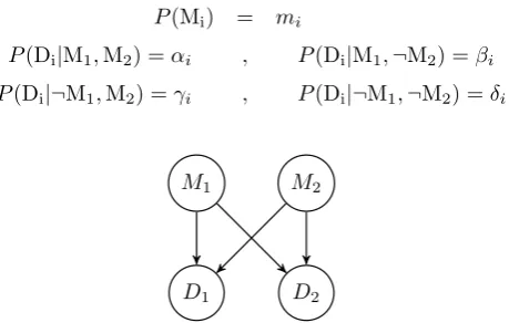
models, M1 and M2, and two pieces of evidence, D1 and D2. This situation is depicted in the Bayesian Network in Figure 1.1 To complete it, we set fori= 1,2:
P(Mi) = mi
P(Di|M1,M2) =αi , P(Di|M1,¬M2) =βi (1)
P(Di|¬M1,M2) =γi , P(Di|¬M1,¬M2) =δi
M1 M2
D1 D2
Figure 1: The Bayesian Network considered in the first step.
Following the discussion in Sec. 4.3, we make four assumptions: (A1) D1 confirms M1. (A2)
D2 confirms M2. (A3) D1 disconfirms M2. (A4) D2 disconfirms M1. Assumption (A1) implies that the likelihood ratio
L1,1:=
P(D1|¬M1)
P(D1|M1) <1. (2)
Assumption (A2) implies that
L2,2:=
P(D2|¬M2)
P(D2|M2) <1. (3)
Assumption (A3) implies that
L1,2:=
P(D1|¬M2)
P(D1|M2) >1. (4)
Finally, assumption (A4) implies that
L2,1:=
P(D2|¬M1)
P(D2|M1)
>1. (5)
1For a straight-forward exposition of the (for philosophical applications) relevant bits and pieces of the theory
of Bayesian Networks, see Bovens and Hartmann (2003: ch. 3).
It is easy to show (proof omitted) that assumptions (A1) - (A4) imply the following two
necessary conditions have to hold ifm1 can take values close to 0 andm2can take values close to 1 (which is reasonable for the situation we consider here): (i)α1, δ1> γ1, (ii)α2, δ2< γ2. We now set
α1=.6 , β1=.4 , γ1=.3 , δ1=.5
α2=.1 , β2=.6 , γ2=.8 , δ2=.4 (6)
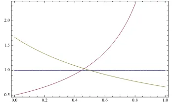
and plot L1,1 and L2,1 as a function of m2 (Figure 2) and L2,2 and L1,2 as a function of m1 (Figure 3). We see that D1confirms M1form2> .25 and that D2disconfirms M1form2> .22. We also see that D2confirms M2 form1< .44 and that D1 disconfirms M2form1< .5.
0.0 0.2 0.4 0.6 0.8 1.0
0.5 1.0 1.5 2.0 2.5
Figure 2: L1,1 (red) andL2,1 (yellow) as a function ofm2 for the parameters from eqs. (6).
0.0 0.2 0.4 0.6 0.8 1.0
0.5 1.0 1.5 2.0
Figure 3: L2,2 (red) andL1,2 (yellow) as a function ofm1 for the parameters from eqs. (6).
Let us now study when the total evidence, i.e. D0 := D1∧D2, confirms M1 and when D0 confirms M2. To do so, we plot
L0,1:=
P(D0|¬M1)
P(D0|M1)
(7)
as a function ofm2 (Figure 4) and
L0,2:=
P(D0|¬M2)
P(D0|M2) (8)
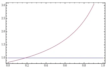
as a function ofm1(Figure 5) for the parameters from eqs. (6). We see that D0confirms M1for
m2 < .18 and that D0 confirms M2 form1 < .18. That is, for m2 > .18, the total evidence D0 always disconfirms M1.
0.0 0.2 0.4 0.6 0.8 1.0 1.0
1.5 2.0 2.5 3.0
Figure 4: L0,1as a function of m2 for the parameters from eqs. (6).
0.0 0.2 0.4 0.6 0.8 1.0
1.0 1.5 2.0 2.5 3.0
Figure 5: L0,2as a function of m1 for the parameters from eqs. (6).
In thesecondstep, we introduce a unifying theory U. U is negatively correlated with M1and positively correlated with M2. This situation is depicted in the Bayesian Network in Figure 6.
To complete this network, we set fori= 1,2
P(U) =u , P(Mi|U) =pi , P(Mi|¬U) =qi, (9)
withp1< q1and p2> q2. To be more specific, let us set
p1=.1 , q1=.4 , p2=.7 , q2=.4. (10)
As mi = u pi + (1−u)qi for i = 1,2, we see that the prior probability m1 decreases from .4 to .1 as u increases from 0 to 1. At the same time m2 increases from .4 to .7. Note that we assume that both models, i.e. M1 and M2, have the same prior probability, viz. .4. That is, in
the absence of a unifying theory, M1and M2 are equally probable.
U
M1 M2
Figure 6: The Bayesian Network considered in the second step.
In the third step, we combine the Bayesian Networks in Figures 1 and 6 and obtain the
Bayesian Nework in Figure 7. The probability distribution is the same as before, i.e. we assume
eqs. (1), (6), (9) and (10).
Figure 8 showsL1,1 andL2,2 (lower two curves) as well asL1,2 andL2,1(upper two curves) as a function ofu. We see that in this part of the parameter space, D1confirms M1, D2confirms M2, D1 disconfirms M2, and D2 disconfirms M1.
U
M1 M2
D1 D2
Figure 7: The Bayesian Network considered in the third step.
0.0 0.2 0.4 0.6 0.8 1.0
1.0 1.5 2.0 2.5
Figure 8: L1,1 (red), L2,2 (yellow), L1,2 (green) and L2,1 (blue) as a function of u for the parameters from eqs. (6) and (10).
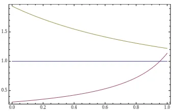
Figure 9 showsL0,1andL0,2as a function ofu. We see that for these parameters, D0always disconfirms M1. We also see that D0 disconfirms M2 for u < .73 and that D0 confirms M2 for
u > .73.
0.0 0.2 0.4 0.6 0.8 1.0
1.0 1.2 1.4 1.6 1.8 2.0
Figure 9: L0,1 (red) and L0,2 (yellow) as a function ofufor the parameters from eqs. (6) and (10).
To complete our discussion, we show that the information setS1:={U,M1,D1}is incoherent
0.0 0.2 0.4 0.6 0.8 1.0 0.5
1.0 1.5
Figure 10: cohS(S1) (red) andcohS(S2) (yellow) as a function ofufor the parameters from eqs. (6) and (10).
whereas the information setS2:={U,M2,D2}is coherent for the parameters used above. To do so, we consider Shogenji’s (1999) measure of coherence, which is defined as follows:
cohS(S1) :=
P(U,M1,D1)
P(U)P(M1)P(D1) (11)
cohS(S2) :=
P(U,M2,D2)
P(U)P(M2)P(D2) (12)
An information set S is coherent if and only ifcohS(S)>1 and incoherent if cohS(S)<1.
Figure 10 showscohS(S1) (lower curve) andcohS(S2) (upper curve) and we see thatS1is (mostly) incoherent whileS2is (always) coherent.
One also sees from Figure 10 that cohS(S1)>1 for large values of u. We take this to be a
misleading artefact of the Shogenji measure which is known to have problems with information
sets of more than two propositions. See Schupbach (2011) for a discussion. Besides Schupbach’s modification of Shogenji’s measure, a more thorough analysis might also want to consider other
coherence measures discussed in the literature. See Bovens and Hartmann (2003) and Schupbach (2011) for references. A more complete analysis will also examine other parts of the parameter
space and derive analytical results. We leave this for another occasion.
1
References
Alais, D., and Burr, D. [2004]: ‘The Ventriloquist Effect Results from Near-optimal Bimodal Integration’, Current Biology, 14, pp. 257-62.
Anderson, J. [1991]: ‘The Adaptive Nature of Human Categorization’, Psychology Review, 98, pp. 409-29.
Angelaki, D.E., Gu, Y. and De Angelis, G.C. [2009]: ‘Multisensory Integration: Psychophysics, Neurophysiology, and Computation’, Current Opinion in Neurobiology, 19, pp. 452-8. Bahrami, B., Olsen, K., Latham, P.E., Roepstorff, A., Rees, G. and Frith, C.D. [2010]: ‘Optimally
interacting minds’, Science, 329, pp. 1081-5.
Baker, C.L., Saxe, R.R. and Tenenbaum, J.B. [2011]: ‘Bayesian Theory of Mind: Modeling Joint
Belief-Desire Attribution’, in L. Carlson, C. Hoelscher and T.F. Shipley (eds.), Proceedings of the 33rd Annual Conference of the Cognitive Science Society, Austin, TX: Cognitive Science Society, pp. 2469-74.
Beauchamp, M.S. [2005]: ‘Statistical Criteria in fMRI Studies of Multisensory Integration’, Neuroinformatics, 3, pp. 93-113.
Bechtel, W. [2006]: Discovering Cell Mechanisms: The Creation of Modern Cell Biology. Cambridge: Cambridge University Press.
Bechtel, W. and Richardson, R. C. [1993]: Discovering Complexity: Decomposition and
Localization as Strategies in Scientific Research. Princeton, NJ: Princeton University Press. Beck, J.M., Ma, W.J., Kiani, R., Hanks, T.D., Churchland, A.K., Roitman, J.D., Shadlen, M.N.,
Latham, P.E. and Pouget A. [2008]: ‘Bayesian Decision Making with Probabilistic Population Codes’, Neuron, 60, pp. 1142-5.
2 BonJour, L. [1985]: The Structure of Empirical Knowledge, Cambridge, MA.: Harvard University
Press.
Bovens, L. and Hartmann, S. [2003]: Bayesian Epistemology, Oxford: Oxford University Press. Bowers, J. S. and Davis, C. J. [2012a]: ‘Bayesian Just-so Stories in Psychology and Neuroscience’,
Psychological Bulletin, 138, pp. 389-414.
Bowers, J. S. and Davis, C. J. [2012b]: ‘Is that What Bayesians Believe? Reply to Griffiths, Chater, Norris, and Pouget (2012)’, Psychological Bulletin, 138, pp. 423-6.
Calvert, G.A. [2001]: ‘Crossmodal Processing in the Human Brain: Insights from Functional
Neuroimaging Studies’, Cerebral Cortex, 11, pp. 1110-23.
Clark, A. [2013]: ‘Whatever Next? Predictive Brains, Situated Agents, and the Future of Cognitive Science’, Behavioral and Brain Science, 36, pp. 181-253.
Colombo, M. and Seriès, P. [2012]: ‘Bayes in the Brain. On Bayesian Modelling in Neuroscience’, The British Journal for Philosophy of Science, 63, pp. 697-723.
Craver, C.F. and Darden, L. [2001]: ‘Discovering Mechanisms in Neurobiology: The Case of Spatial Memory’, in P. K. Machamer, R. Grush, and P. McLaughlin (eds.), Theory and Method in the Neurosciences. Pittsburgh, PA: University of Pittsburgh Press, pp. 112-37.
Danks, D. [2007]: ‘Theory Unification and Graphical Models in Human Categorization’, in A. Gopnik and L. Schulz (eds.), Causal Learning: Psychology, Philosophy, and Computation. New York: Oxford University Press, pp. 173-89.
Darden, L. [2006]: Reasoning in Biological Discoveries. Cambridge: Cambridge University Press. Darden, L. and Craver, C. F. [2002]: ‘Strategies in the Interfield Discovery of the Mechanism of
Protein Synthesis’, Studies in History and Philosophy of Biological and Biomedical Sciences,
33, pp. 1-28.
Deneve, S. [2008]: ‘Bayesian Spiking Neurons i: Inference’, Neural Computation, 20, pp. 91-117. Eberhardt, F. and Danks, D. [2011]: ‘Confirmation in the Cognitive Sciences: The Problematic