Issues
ISSN: 2146-4138
available at http: www.econjournals.com
International Journal of Economics and Financial Issues, 2016, 6(S2) 138-150.
Special Issue for “State and Municipal Regulation, Investment, Commerce: National and International Aspects of the Business”
Economic Estimation of Project Risks when Exploring Sea Gas
and Oil Deposits in the Russian Arctic
Marina Nikolayevna Kruk
1*, Anni Yulievna Nikulina
21National Mineral Resources University (Mining University), 21 Linia 2, 199106 Saint Petersburg, Russia, 2National Mineral
Resources University (Mining University), 21 Linia 2, 199106 Saint Petersburg, Russia. *Email: [email protected]
ABSTRACT
The aim of the article is to develop the methodology of economic estimation of risks when exploring shelf deposits of the Ob Bay in the Arctic Region of Russia. It considers various methods of accounting and economic estimation of risks: Sensitivity analysis, scenarios method, imitation modeling, and the method of real options. Calculations and the conclusion about the most rational method for calculating sea Arctic projects were made. This method of real options allows to take into account peculiarities of venture projects. This work is practically important because the offered methodology can be applied for all gas-and-oil deposits at the Arctic shelf of Russia that have been actively developed over the last decade.
Keywords: Risk, Option, Oil, Gas, Shelf, Deposit, Sensitivity Analysis JEL Classifications: Q32, Q39, Q47
1. INTRODUCTION
Over a recent decade due to a number of unique gas-and-oil deposits the Arctic Region of the Russian Federation has been attracting a great attention of Russian and foreign extracting companies. In spite of the temporary decrease in prices for hydrocarbons on the world market related to political reasons more than to economic regulation, the shelf deposits of the Russian Arctic are promising for the exploitation in the coming decades. “Energy Strategy of Russia up to 2030” proves this. So, in case of stabilization of the price for oil on the level of USD 100 per barrel, it is possible to speak about the reasonability to introduce large-scale projects of gas and oil exploration in the Arctic shelf of Russia (Kursky and Kurskaya, 2001; Cherepovitsyn et al.., 2012).
Today the first developing Arctic deposit is Prirazlomnoye in the Pechora Sea. Oil started appearing from it in 2014. However, in the future it is planned to explore other deposits, too (Facts. The Norwegian Petroleum Sector, 2014; Smith and Lalwani, 1991; Azarnov, 2001).
The group of deposits located in the Ob Bay of the Kara Sea is extremely promising for exploration. This group includes such deposits as Severo-Kamenomysskoye, Kamenomysskoye-more and Chugoriahinskoye deposits (Figure 1). The deposits of this group are located in the basin of the Ob Bay of the Kara Sea. The depth of the sea in this area is approximately 6 m (Bobylev, 2006; Gasprom and OJSC, n.d.).
However, due to natural and climate, technical and technological, financial and other difficulties, Arctic gas-and-oil projects are extremely risky. In order to objectively estimate all possible risks and develop the program of their leveling, it is necessary to develop special tools (Zakharov, 2002; Zakharov and Nikitin, 2003; Zakharov and Kholodilov, 2002; Zakharov et al., 2004; Kostenko, 2009). Generally risks estimation is the process of defining the probability of occurrence of risk factors - specific events or situations that can affect the development of the project (business) and achievement of the target results.
analysis), and quantitative estimation of the damage from their occurrence (quantitative analysis) (Berlin et al., 2003a; Berlin et al., 2003b; Grigorenko, 2006).
The task of the qualitative analysis of risk is to reveal the sources and reasons of risk, stages and works whose performance is assisted by risks, i.e.:
• Determining potential zones of risk
• Revealing risks associated with the enterprise activity, and • Forecasting practical benefits and possible negative
consequences of the revealed risks occurrence.
The main task of this stage of estimating gas-and-oil projects is to reveal basic types of risks that influence financial and economic activity of the gas-and-oil producing complex.
2. METHODOLOGY
It is offered to use the following methods of research for economic estimation of risks: Sensitivity analysis (2.1), imitation
modeling (2.2), scenarios method (2.3), and real options method (2.4) (Volkov, 2007; Gert et al., 2008; Kozlovskaya, 2009; Ecological Risks When Producing and Transporting Raw Hydrocarbon. Yamal did not approve the construction of Gazprom’s underwater gas Pipe 2010, April 02).
2.1. Economic Estimation of Project Risks Based on the Sensitivity Analysis
Sensitivity analysis is made for accounting and forecasting the influence of changing input parameters (investment expenditures, cash flow, cut-off rate, re-investments level) of the investment project on the resulting indicators (Gracheva, 2009; Gracheva and Sekerin, 2012).
The most convenient variant is relative change of one of the input parameters (example - All cash flows minus 5%), and analysis of the changes that took place in the resulting indicators.
The main thing for the sensitivity analysis is to estimate the level of influence of every input parameter change in order to foresee
the worst development of the situation in the business plan (investment project).
The formula to compare input parameters with the ones calculated according to the data of the sensitivity analysis (Koshechkin, 2009a), (Formula 1) is the following:
100%
sa in
in
A A
A A
−
∆ = ⋅ (1)
ΔА - The value change in %
Аin - The initial (primary) value of the A parameter
Аsa - Parameters calculated according to the data of the sensitivity analysis (A target value).
The aim of the analysis is to determine the level of influence of separate changing factors on financial indicators of the investment project. Its tools allow to estimate potential impact of the risk on the project efficiency.
The sensitivity analysis defines investment criteria for the large scale of initial conditions. The most important parameters of the project are singled out, and regularities of the change of financial results from the dynamics of every parameter are revealed.
When researching the sensitivity of the capital project, the following parameters are usually considered:
a. Physical volume of sales as a result of the market capacity, share of enterprises on the market, potential of the market demand growth
b. Product (service) price c. Inflation rate
d. Required volume of capital investments e. Need in floating capital
f. Variable expenses g. Standing costs
h. Refinancing rate of the percent for the bank credit, etc. These parameters cannot be changed by taking management decisions.
In the process of analyzing sensitivity, “basic” variant is defined. Under it all parameters under research acquire their initial value. Only after that, the value of one of the researched factors varies in the specific interval under stable values of other parameters. Besides, the sensitivity analysis is the basis for the project acceptance. So, for example, if the price happened to be a critical factor, it is possible to strengthen the marketing program or reconsider the expense component of the project in order to decrease its cost.
The sensitivity indicator is calculated as the relation of the percent change of the criteria - The selected indicator of the investments efficiency (in relation to the basic variant) to the change of the factor by one percent. Sensitivity indicators for every factor under research are defined in such a manner.
Using the sensitivity analysis and being based on the received data, it is possible to determine the most top-priority factors in terms of risk, and to develop the most efficient strategy of the investment project implementation.
There are two basic methods of the sensitivity analysis that do not contradict each other. That’s why they can be applied both together and separately. They include the following methods.
2.1.1. Pivot points method
It is based on searching for such value of the factor indicator under which the resulting criteria is zero. The critical level of the factor indicator revealed in such a manner is equal to its forecasting value. The less difference between the critical and forecasting levels is, the higher sensitivity of the criteria in relation to this factor is, because the probability of its achievement of the critical point is higher. Typical examples of critical points include IRR - according to the “profitability of the alternative investment” factor, BEP breakeven point - according to the “production volume” factor, and payout time - according to the “life of project” factor (Limitovskiy, 2004).
The analysis comes down to the determination of the reality of the situation under which the parameter will achieve its critical point. The more probable such situation is, the more attention it is necessary to pay to this parameter, try to insure against its changes with the aid of various warrants, make a more detailed research on its clarifying, etc.
2.1.2. Method of sustainable ranges or dependences
In this case a specific range of changes in the factor indicator is chosen, and based on this interval the dependence of the resulting criteria (net present value [NPV]) on it is made.
Parameters in relation to which the NPV elasticity is maximum are thought to be the riskiest.
Either of these two parameters allows to reveal the most important factors that influence the result of the project, timely waive it or to take measures on efficient management and control over the risk taking into account parameters that are maximally exposed to risk (Kendrick, 2015).
Algorithm to analyze sensitivity by sustainable ranges method: Step 1: Defining key variables that have an impact on the NPV
value.
Step 2: Defining analytical dependence of NPV on key variables.
Step 3: Calculation of basic situations - Defining the expected value of NPV under expected values of the key variables.
Step 4: Changing one of the input variables to the volume (%) required by the analyst. Herewith, all other input variables have fixed values.
Step 5: Calculating a new value of NPV and its change in percent.
Step 6: Calculating critical values of variables of the project and defining the most sensitive of them.
Step 7: Analyzing the received results and forming NPV sensitivity to changing various input parameters. Critical values of the indicator are the values when the current cost is zero (NPV =0).
2.2. Imitation Modeling
In the contemporary literature there is no unified opinion about defining imitation modeling. So, there are various interpretations (Koshechkin, 2009a; Koshechkin, 2009b):
• Firstly, the imitation model is understood as a mathematical model in its classical sense.
• Secondly, this term is maintained only for those models where random influences happen (are imitated) in any manner. • Thirdly, the imitation model if thought to differ from an
ordinary mathematical model by more detailed description; however, no criterion that witnesses about the end of the mathematical model and the beginning of an imitation model is introduced.
Imitation modeling is applied to the processes that can be from time to time interfered with the human will. The person who manages the operation may take various decisions depending on the current situation. Then the mathematical model is brought into operation. It shows what change of the situation as a response to this decision is expected and what will be the consequences in some time. The next current decision is made taking into account the real new situation, etc.
Algorithm of imitation modeling:
Step 1: Creating a forecasting model in the mode of Excel table editor.
Step 2: Setting the function of allocating every variable that has an impact on forming the cash flow and introducing its minimum and maximum values. For this purpose we assign the probable allocation to the variable based on the estimates or our expectations (for example, the triangular, normal or equal allocation).
Step 3: Carrying out calculation iterations that is an entirely computerized part of the project risks analysis. Usually 200-500 iterations are enough for a good representative sample.
In the process of every iteration, there is a random selection of values of key variables from the specified interval in accordance with the probable allocations and correlation conditions. Then resulting indicators (for example, NPV) are calculated and maintained. Step 4: Carrying out statistical analysis of the received results
and making a histogram of allocating the resulting indicator. Using it, it is possible to estimate the risk of the project and variance of possible results. 2.3. Scenarios Method
When developing management decisions, the scenarios method is widely used. It allows to estimate the most probable process in
the course of events and potential consequences of the decisions that are taken.
To various confidence degrees, the scenarios of the development of the situation under analysis developed by specialists allow to determine possible tendencies of the development and interrelation between the current factors, to form the picture of possible states the situation may have under the influence of various impacts. On the one hand, professionally developed scenarios allow to more fully and clearly define the perspectives of the situation development under both the occurrence and the absence of various management impacts.
On the other hand, scenarios of the expected development of the situation allow to timely realize the dangers unsuccessful management impacts or unfavorable course of events are fraught with.
The comparison and the estimation of possible scenarios of the situation development under the influence of both various management impacts and background factors that do not depend on actions contribute to making only right choices.
The scenarios method assumes the creation of technologies related to the development of scenarios that ensure higher probability of working out an efficient decision in those situations when it is possible, and higher probability of minimizing the expected losses in those situations when losses are inevitable.
At the present time various methods to implement the scenarios method are known (Koshechkin, 2009a; Kruk, 2012a; Kruk, 2012b); They include:
• Method of receiving the agreed opinion is essentially one of the realizations of the Delphi method focused on the receipt of the collective mind of various groups of experts in relation to serious events in various areas for the determined period of future.
It is possible to specify such drawbacks of this method as insufficient attention paid to the interdependance and interrelation of various factors that influence the course of events and dynamics of the situation development.
• The method of recurrent combination of independent scenarios lies in composing independent scenarios for every aspect that considerably influences the development of the situation and recurrent iterative process of agreeing scenarios of the development of various aspects of the situation.
The advantages of this method include the deepened analysis of the interrelation of various aspects of the situation development. Its disadvantage is a weak status and methodological provision of procedures related to scenarios agreement.
However, when estimating innovational projects that are influenced by special risks that are specific for this project, it is necessary to use the improved approach to undertaking the scenarios analysis. Algorithm to estimate risks by scenarios method:
Step 1: Creating the forecasting model in the mode of the Excel table editor.
Step 2: Defining key factors using the sensitivity analysis by the fiducial points method.
Step 3: Defining correlation dependence between these parameters.
Step 4: Analysis of forecasts of the leading institutes and companies in the energy area. The number of institutes and companies must be equal. The use of the equal number will allow to achieve more accurate forecasting because the estimates of gas-and-oil companies are usually a little bit overstated, and the estimates of institutes are on the contrary under-valuated.
Step 5: Defining the influence of forecasts on the project key factors.
Step 6: Composing scenarios on the basis of the obtained information.
As a rule, data about several possible scenarios of the situation development are more informative than one scenario, and contribute to taking more efficient decisions.
2.4. Method of Real Options and Opportunities to Apply it in Risks Management
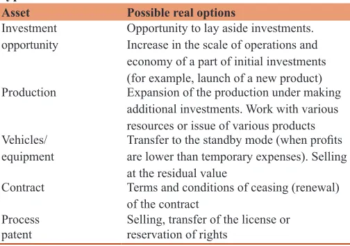
In many cases the management can take decisions during project development in order to increase its profitability. So, in case of the situation worsening, it is possible to stop or cease the project. With luck, it is possible to grow the capacities, increase the scales of the project for receiving more profits. In case the situation is indefinite, it is possible to lay aside basic initial investments and support only the possibility of their quick effectuation when favorable events occur. Anyhow, a lot of investment projects are flexible. It is natural that such right to influence the investment process has its definite cost. The real options method, first of all, focuses on determining the cost of this right, defining the cost of the real options built-in in the project (Bruslanova, 2004; Gracheva, 2009; Gracheva and Sekerin, 2012).
The notion of real option is determined as the right of its owner, but not the obligation, to make a specific action in the future. Financial options provide the right to buy (sell) a specific basic asset and insure financial risks. Real options entitle to change the process of the project implementation and insure against strategic risks. As a rule, real options are identified with a specific asset of the company, for example, a patent or license. The patent or license for the product provides the firm with the right to develop the product and its market. Owing a patent, the firm can start selling the product at any moment by having made initial investments in its development.
The real options method assumes an essentially new approach. The indefiniteness remains, and with the course of time management
adjusts (takes optimal decisions) to the changing situation. In other words, real options offer the opportunity to change and take optimal decisions in the future in accordance with new information that is received. Herewith, opportunities to take and change decisions in the future are estimated in a qualitative manner during the analysis. It is necessary to note that regardless of the chosen method of the investment project estimation, in the majority of cases the management has an opportunity to take optimal decisions and change the ones that have already been taken. The problem of the method of discounting cash flows lies in the fact that it does not take into account such opportunities at the stage of estimating the efficiency of the investment project.
It is reasonable to apply the real options method to the estimation of investment projects when the following conditions are complied with:
• The result of the project undergoes a high level of indefiniteness • The company management can take flexible management
decisions when new data on the project occurs, and
• To a great degree the financial result of the project depends on the decisions taken by the management.
Depending on the conditions under which the option acquires significance for the company, the following basic types of real options are distinguished (Bruslanova, 2004; Zubareva et al., 2005). The first option is the possibility to delay. The delay occurs when the company can postpone the decision about basic investments till some moment in the future, and decrease the project risk in such a manner. Herewith, in case of a delay the company must possess relatively unique assets in order to be sure that other companies will not take up its niche and make investments earlier (patents, proper developments and unique technologies offer such opportunity).
The second option is one of the most wide-spread ones. This is the possibility to change the project scale. The option lies in the fact that the management can increase or decrease the project scale. Accordingly under favorable situation (growth of clients, demand for products, etc.) additional funds can be invested in the project. And in case of the situation worsening, the project can be decreased till the reduction of incremental cost has a positive impact on the profit. Such option can be valuable in the industries that are exposed to cyclic development under which a decline in production intersperses with its sharp growth.
In our case the basic asset is the successive deposit. The price of exercising is the required additional investments. The price of the basic asset is equivalent to the cost of the cash flows adjusted to the moment of the option exercising. The term of exercising the option is the term during which it is possible and economically reasonable to expand the capacities.
If the probability of success is Psuccess, the expected net discounted profit will be equal to,
Where NPVexpectis the expected value of the net discounted profit, monetary unit.
NPVoptionis the value of the net discounted profit when using the expansion option, monetary unit. This value is received after overlaying additional flows related to additional investments and additional profits on the initial cash flows.
NPVwithout optionis the value of the net discounted profit without using the expansion option (variant when the expansion is considered unreasonable), monetary unit.
Psuccess is the probability of success, %.
The cost of the expansion option is defined according to the following formula:
Poption = NPVexpect – NPVwithout option (3) Where Poption is the cost of the management option, monetary unit. The third option - an output option - allows the company to refuse from implementing the project in case of a sharp worsening of the market environment. Then the company can sell assets to a third party and compensate for a part of its losses, or use them in other investments.
If the probability of negative course of events is Pneg., the expected value of the net discounted profit without using the outflow option will be:
with
expect. neg neg pos pos
NPV =P ×NPV +P ×NPV (4)
Where NPVneg is the value of the net discounted profit in case of negative course of events, monetary unit
NPVpos is the value of the net discounted profit in case of positive course of events, monetary unit
Pneg is the probability of negative course of events, %
Ppos is the probability of positive course of events, %.
If the management can stop the project, the value NPV in case of negative course of events must be replaced by the project cost in case of its liquidation.
The value of the expected net discounted profit when using the output option is calculated according to the following formula:
option option
expect neg neg pos pos
NPV =P ×NPV +P ×NPV (5)
Where NPVnegoptionis the value of the net discounted profit in case of negative course of events and using the outflow option, monetary unit.
The cost of the outflow option is calculated similarly to the cost of the expansion option.
The profit from implementing the project taking into account management options is equal to the sum of profits within the traditional methodology (NPV) and cost of all management options (in this case this is expansion and outflow options).
Table 1 shows examples of possible real options in relation to various types of assets.
In respect to investment projects in the sea gas-and-oil industry, the use of the real options method somehow differs from the one generally accepted, and has a number of specific peculiarities because these projects are implemented according to several stages. The duration of the investment project implementation is rather long. The difficulty lies in the fact that it will not be possible to apply the standard sample in this case. It is necessary to create the model that will specify what options can be applied at what stages of the deposit exploration. When estimating risks, the binary tree of scenarios of the investment project development is made. Figure 2 shows the model of such multi-component tree of scenarios. The white color shows optimistic scenarios, and blue color demonstrates pessimistic ones, i.e., the ones when risks are realized.
The first component of the tree is represented by two issues A1 and A2, the second - four issues B, the third - eight issues C, etc. Every branch is assigned with specific probability that the next event will occur under the condition that the previous event occurred. Depending on the structure, the tree units may include the value of the project (then this is a value tree), its cash flows (then this is a cash flows tree), or the option value (then this is an option tree) (Limitovskiy, 2004).
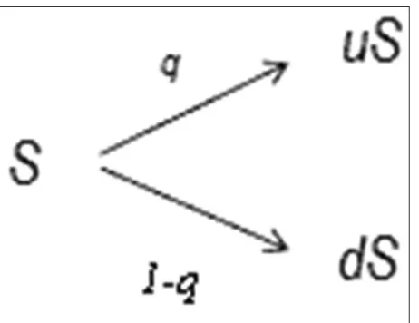
The binominal model means the determination of the option cost on the basis of constructing the tree of changes of the cost of the basic asset in time by using the raising (u) and descending (d = 1/u) coefficients. It is supposed that S is the cost of the basic asset at the time t0, and at the time t1 it will be equal to u·S with the probability q, and d·S with the probability (1−q) (Figure 3).
The receipt of these values allows to make the decision about exercising or non-exercising of the option and to find possible values of option payments at the time t1.
Table 1: Examples of real options in relation to various types of assets
Asset Possible real options
Investment
opportunity Opportunity to lay aside investments. Increase in the scale of operations and economy of a part of initial investments (for example, launch of a new product) Production Expansion of the production under making
additional investments. Work with various resources or issue of various products
Vehicles/
equipment Transfer to the standby mode (when profits are lower than temporary expenses). Selling
at the residual value
Contract Terms and conditions of ceasing (renewal)
of the contract
Process
Figure 3 shows the change of the cost of the basic asset, replicating portfolio, dependence of the option cost on possible payments at the end of the period t = 1.
The u and d values are defined on the basis of the supposition that the change of the price of the basic asset can be described by the geometrical Brownian motion, and are found according to the following formulae:
u e= µτ σ τ+ , (6)
d e= µτ σ τ− , (7)
Where,
µ is the average speed of the price trend expressed as a simple annual percent.
Figure 2: Binary tree of scenarios to develop investment project (Kruk, 2012a; Kruk, 2012b)
σ is the volatility.
τ is a step expressed in the shares of a year. On average, 1 year is equal to 252 working days and if, for example, step in time is equal to 1 day (ordinary case), τ=1/252.
Thus, when estimating the project, the calculation algorithm will be as follows:
1. We will estimate the speed of the trend and volatility of prices. The volatility is defined according to the prices of the basic asset at some proceeding period of time. In order to get the estimation of µ, σparameters according to the discrete set of prices of the basic asset F0= F, F1, F2, ... Fm, it is necessary to define relative changes of the price for the period.
1 0 2 1 1
1 2
0 , 1 , , 1
m m
m m
F F F F F F
u u u
F F F
−
−
− − −
= = … = (8)
To calculate the average speed of the trend:
1 2 m,
u u u
u
m + + ⋅⋅⋅ +
= (9)
And then calculate the estimation of volatility for the period τ:
2 2 2
1 2
( ) ( ) ( )
1 m
u u u u u u
m
δ = − + − + ⋅⋅⋅ + −
− (10)
µ, σ coefficients are estimated by standardizing: µ υ
τ
= σ = δτ (11)
2. Using the DCF method, we will estimate cash flows from the project applying the risk free rate. In order to decrease calculations, we will focus on the opinion of Limitovskiy, and consider the risk-free rate as equal to the rate of the percent for state bonds (6.25%).
3. We will determine the increasing (u) and decreasing (d) coefficients, the profit that will be received by the option owner in case of the optimistic variant (Сu), the profit eaned in case of the pessimistic variant (Cd), and the risk neutral probability р.
1 Rf d p
u d
+ −
=
− (12)
4. Herewith, the price of the option can be defined as:
(1 ) 1
u d
f
pC p C
C
R + − =
+ (13)
Where Сu is the profit that will be earned by the option owner in case of the optimistic variant; Сu = uV0 -X
Cdis the profit earned in the pessimistic variant
Rf is the risk free rate of the discount.
With the mentioned schemes and algorithms, when estimating risks of the investment project in the gas-and-oil industry, it is possible
to more accurately define the amount of the reported profit from the project implementation.
3. RESULTS
3.1. Analysis of Sensitivity of Project Efficiency
Indicators
It was decided to conduct the sensitivity analysis by using two existing methods in combination, because the method of pivot points defines the factors that are most sensitive to the occurrence of the risk situation, and the method of rational ranges vividly shows the result of the dependence of the resulting indicator on changes of key (Gracheva and Sekerin, 2012).
3.1.1. Pivot points method
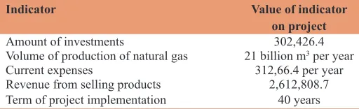
Let’s consider the basic factors that influence the efficiency of the investment project related to exploring the Kamenomysskaya group of deposits. Table 2 shows the basic data related to the project.
Having estimated the value of NPV for the project, using the “decision search” function, we will find the initial values of basic factors when NPV of the project is 0.
Having conducted the sensitivity analysis according to the pivot, we have obtained the following results (Table 3).
Thus, the project is sensitive to almost all factors risks. However, the effect from the project shows the greatest sensitivity to the market (current expenses and revenues) and technical (production volume) estimates. It means that not only marketing estimates of the market, first of all forecasts of prices for gas, but also technological provision of the project functioning are important for this project. That’s why when forming the strategy of the project risks management, it is necessary to pay the greatest attention to the market, operational and technological risks.
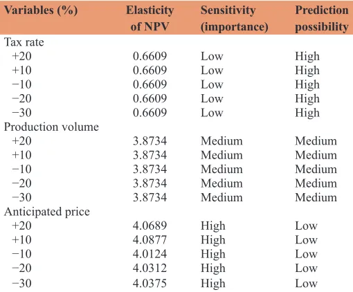
3.1.2. Method of sustainable ranges or dependences
In order to analyze sensitivity using this method, it is necessary to define key indicators that influence the factors of successful implementation of the project. When exploring the deposits of the Ob Bay, such factors include the tax rate, the production volume, and the expected price from selling natural gas. We will change these indicators in the range from −30% to +20% and find NPV for every change. We will estimate the NPV elasticity when these parameters are changed (Table 4) and represent the obtained data as a graph (Figure 4), where the Х-axis shows the change of the basic parameter in %, and the Y-axis shows the value of NPV under the changed meaning of the parameter.
Table 2: Basic data on project, million RUB
Indicator Value of indicator
on project
Amount of investments 302,426.4
Volume of production of natural gas 21 billion m3 per year
Current expenses 312,66.4 per year
3.2. Risk Analysis of the Investment Project by the Scenarios Method
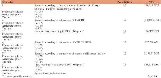
The present work considers possible scenarios of the investment project implementation. For this we determined the key factors of the project that have a considerable impact on the efficiency indicator - NPV. In this case these factors include taxes rates, production volume and product price.
In the research we analyzed economic scenarios of the development of such scientific establishments and commercial companies as the Energy Research Institute of the Russian Academy of Sciences, TNK-BP, PJSC Gazprom, VTB CAPITAL, Institute for Energy and Finance, and we made the calculation according to the scenario “tax vacations” of PJSC “Gazprom” (Alekperov, 2010; Newsletters of Fuel and Energy Complex, 2009; Gasprom and OJSC, n.d.).
Having analyzed the forecasts of various institutes and companies in the power industry, it is possible to single out the following most probable scenarios of the course of events for the considered project of exploring the deposits of the Ob Bay (Table 5). The conducted economic and statistical analysis of the project (Table 6) allows to make the following conclusions:
1. The most probable NPV of the project (RUB 176,435.4 million) is a bit higher than it is expected from its implementation (RUB 174,619.4 million).
2. The probability to get NPV below zero is 17%. The project has rather high spread in values of NPV indicator. This is proved by the coefficient of variation and the value of the standard deviation, and characterizes the project as rather risky. Herewith, the decrease in the production volume and price of selling are non-doubtful factors of risk.
3. In accordance with the three sigma rule, the price of the investment project risk is RUB 3*20,204.02 = 60,612.06 million It does not exceed the most probable NPV of the project (RUB 176,435.4 million).
The risk price can be also characterized through the indicator of the variation coefficient. In this case the coefficient of variation =0.10. It means that 10 kopeikas of possible losses occur per a ruble of the average profit (NPV) from the investment project.
Thus, in spite of the fact that the project riskiness is high, the development of this project is rather reasonable.
3.3. Risk Analysis of the Investment Project by the Imitation Modeling Method
Based on the results of the analysis, the most important variables were selected, and NPV values were received according to three
Table 4: Indicators of sensitivity and predicted variables in project
Variables (%) Elasticity
of NPV Sensitivity (importance) Prediction possibility Tax rate
+20 0.6609 Low High
+10 0.6609 Low High
−10 0.6609 Low High
−20 0.6609 Low High
−30 0.6609 Low High
Production volume
+20 3.8734 Medium Medium
+10 3.8734 Medium Medium
−10 3.8734 Medium Medium
−20 3.8734 Medium Medium
−30 3.8734 Medium Medium
Anticipated price
+20 4.0689 High Low
+10 4.0877 High Low
−10 4.0124 High Low
−20 4.0312 High Low
−30 4.0375 High Low
NPV: Net present value
Table 3: Sensitivity for risk factors of the project on exploring the Kamenomysskaya group of deposits
Risk factor Anticipated value on project Critical value (pivot point), million RUB Critical change (%)
Amount of investments, million RUB 302,426.4 525,980.8207 73.9
Production volume, billion m3 840 718.85 −14.4
Current expenses, million RUB 1,250,656 1,699,122.963 35.8
Discount rate 10% 16.4% 64
Income tax 20% 37.5% 87.5
Revenue, million RUB 2,612,808.7 2,164,341.74 −17.2
Figure 4: Changing the net present value of the project on exploring the kamenomysskoye group of deposits when changing resulting factors
According to the results of the conducted research, it is possible to make the following conclusion:
supporting variants of the course of events (the best, the worst, basic). Using the method of expert estimates, the probabilities to implement these variants were defined. The obtained results were used as initial data for the imitation modeling (Table 7).
Being based on the initial data, we will conduct imitation. In order to do so, it is recommended to use normal allocation, because the practice of risk analysis showed that it had been observed in the vast majority of cases. The number of imitations can be any and is determined by the required accuracy of the analysis. In this case we will be limited to 500 imitations.
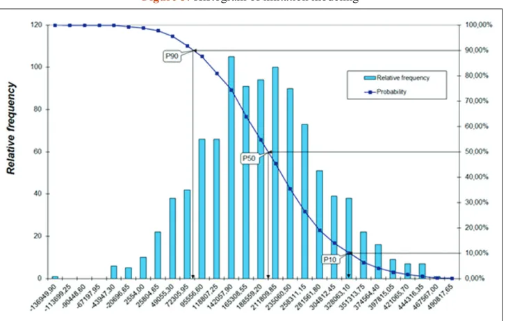
When making the Monte Carlo model, we used 5 variables that were revealed as a result of the sensitivity analysis. Figure 5 graphically shows the results of estimating the indicator NPV by the Monte Carlo method.
Based on the data received as a result of imitation, using standard functions of MS Excel, we will make economic and statistical analysis (Table 8).
Imitation modeling showed the following results:
1. The average value of NPV is RUB 179,153.06 million 2. The minimum value of NPV is RUB 136,949.9019 million 3. The maximum value of NPV is RUB 490,817.82 million 4. The coefficient of variation of NPV is 52%
5. The number of cases of NPV<0-19
6. The probability that NPV will be below zero is 0.019 7. The probability that NPV will be above the maximum is zero 8. The probability that NPV will be in the interval [M(E)+s;
Max] is 16%
9. The probability that NPV will be in the interval [M(E)−s; M(E)] is 34%.
In order to calculate the price of risk in this case, we use the indicator of the mean-square deviation - s, and mathematical expectation - М (NPV). In accordance with the three sigma rule, the random value, in this case - NPV, is in the interval [М−3s; М+3s] with the probability that is close to 1. In the economic context this rule can be interpreted as follows:
• The probability to get NPV of the project in the interval [179,153.06−94,035.74; 179,153.06+94,035.74] is 68%, • The probability to get NPV of the project in the interval
Table 5: Scenarios of developing project on exploring the Kamenomysskoye group of deposits (Kruk, 2012a; Kruk, 2012b; Limitovskiy, 2004)
Scenarios Probabilities NPV
1 Scenario according to the estimations of Institute for Energy
Studies of the Russian Academy of sciences 0.2 154,253.2072
Production volume +11.5% Anticipated price +9.7%
Tax rate +5.3%
2 Scenario according to estimations of TNK-BP 0.2 −38,071.24128
Production volume −21.5% Anticipated price −12.8%
Tax rate +6.8%
3 Basic scenario according to CJSC “Gasprom” 0.1 174619.3559
Production volume Anticipated price Tax rate
4 Scenario according to estimations of VTB CAPITAL 0.2 377,790.478
Production volume +13.7% Anticipated price +11.3%
Tax rate −12.1%
5 Scenario according to estimations of energy and finances institute 0.2 3,351.972457 Production volume −15.7%
Anticipated price −11.6%
Tax rate −15.8%
6 “Tax vacations” scenario of CJSC “Gasprom” 0.1 353,834.2505
Production volume +7.8% Anticipated price +9.7%
Tax rate Special terms and conditions
The most probable scenario 176,435.4
Table 6: Economic and statistical analysis of results
Indicator Value
The most probable value NPV 176,435.4
Deviation 20,204.02
Variation coefficient 0.10
P (NPV<=0) 0.17
P (NPV<average−10%) 0.33
P (NPV>average+10%) 0.50
NPV: Net present value
Table 7: Key parameters of project
Indicators Indicator value
Minimum Maximum
Volume of natural gas production, billion m3
588 1,008
Income on selling products,
million RUB 2,707,897.29 4,642,109.64
Taxes and payments,
million RUB 102,132.072 175,083.552
Amount of investments,
million RUB 211,698.83 362,912.28
Exploitation expenses,
[179,153.06−188,041.48; 179,153.06+188,041.48] is 94%, and,
• The probability to get NPV of the project in the interval [179,153.06−282,107.22; 179,153.06+282,107.22] is close to one, i.e., the probability that the value of NPV of the project will be less than RUB 179,153.06 million (179,153.06−282,107.22) goes to zero.
So, the sum of the possible losses that characterize this investment project is RUB 282,107.22 million (it allows to speak about the high level of riskiness of this project).
In other words, the price of risk of this investment project is RUB 282,107.22 million of conditional loss, i.e., the acceptance of this investment project causes the possibility to lose not more than RUB 282,107.22 million.
4. DISCUSSION
4.1. Sensitivity Analysis
It is necessary to note that in spite of all advantages of the method of the project sensitivity analysis, including objectivity, simplicity
of calculation, their demonstrativeness (these criteria are put into the basis of its practical use), this method has a serious disadvantage - its mono-factor nature. It focuses only on changing one factor of the project. It results in the undercount of opportunities of the relation between separate factors or undercount of their correlation. Along with this, the change of some indicators leads to changes of other indicators (for example, a growth of expenses leads to a change of prices that leads to a decrease in the demand for goods and volume of sales, etc.). That’s why some researches find it reasonable to model internal interrelations between the project parameters, and it is done using the Monte Carlo method. Nevertheless, the Monte Carlo (imitation modeling) method cannot be thought to be optimal. Imitation modeling according to the Monte Carlo method has the following disadvantages:
• In the process of modeling internal interrelations there is much routine work, and it becomes a hard task to compose the system that does not contradict them.
• Due to the availability of a great number of such relations, the decision happens to be unstable.
• The interrelations of phenomena and errors of the forecasting themselves as well as expected allocations of probabilities according to basic parameters are made with the involvement of expert information. That’s why an increase in the labor intensity of calculations is not always assisted by an adequate increase in its accuracy.
As for the scenarios method presented in the work, its disadvantages may include the labor intensity of getting a great number of estimates and their correct processing. Control actions lead to the shift of the system position in the space of parameters. In this case it is also reasonable to consider only discrete points, and herewith to pay the greatest attention to the most probable points. Under such analysis it is necessary to foresee the possibility of occurrence of additional internal tensions between the system elements, because they can also change the system position in the space of parameters.
Figure 5: Histogram of imitation modeling
Table 8: Economic and statistical analysis of imitation results
Indicator Value
Average value 179,153.06
Standard deviation 94,035.74
Variation coefficient 0.52
Minimum −136,949.9019
Maximum 490,817.82
Number of cases NPV<0
P (E<=0) 19
P (E<=Min(E)) 0.00
P (Е>Max(E)) 0.00
P (M(E)+s<=E<=Max) 16.00
P (M(E)−s<=E<=M(E)) 34.00
If we speak about the method of estimating risks with the aid of real options, under the current conditions for Russia it is almost not applied due to legal and judicial peculiarities of the legislation. That’s why it was decided not to include this method in the general comparative analysis of the methods related to estimating quantitative risk.
Comparative Table 9 was made on the basis of the risks estimation methods under analysis.
5. CONCLUSION
As a conclusion, we would like to note that the offered methods used for risk estimation characterize the risks in terms of the impact of factors of inner and outer circle on the target indicator of the estimation of the investment project efficiency. In the present work we have made a detailed analysis of the methods that are the most actively used, developed algorithms of applying these methods, and offered the modification of the scenarios method. The latter means more serious working out of the obtained data and development of the most probable forecasts. Further work at this theme assumes full comprehensive estimation of the risk that includes such stages as identification, quantitative and qualitative estimation of possible damage as well as selection of the risks management method and determining the combination of measures required for decreasing the risk level and minimizing the supposed damage.
REFERENCES
Alekperov, V. (2010), It Is Necessary to Share Risks. Shelf Resources. p19-21.
Azarnov, A. (2001), On Russian and Norwegian legislation in the gas-and-oil producing industry. Oil, Gas and Law, 3(39), 29-35. Berlin, A., Berlin, A.I., Vrooman, L.L.P. (2003a), Managing political risk
in the oil and gas industries. OGEL Journal Oil, Gas and Energy Law Intelligence, 1(2), 1-17.
Berlin, A., Berlin, A.I., Vrooman, L.L.P. (2003b), Types of coverage and measure of loss. OGEL Journal Oil, Gas and Energy Law Intelligence, 1(2), 8-12.
Bobylev, V.N. (2006), On categories of reserves and resources. Oil, Gas and Capital Market, [Date Views: 13.03.2016]. Available from: www. ngfr.ru/article.html?011.
Bruslanova, N. (2004), Estimation of investment projects by real options method. Financial Director, 7. [Date Views: 13.03.2016]. Available from: http://fd.ru/articles/10485-red-metod-realnyh-optsionov-v-otsenke-investitsionnyh-proektov.
Cherepovitsyn, A.E., Nikulina, A.Y., Sheikin, A.G. (2012), Interrelation of companies and state when implementing large-scale projects on developing sea shelf: Opportunities of small business. Vol. 9. Contemporary Economy: Problems and Solutions. Voronezh: (Publishing House of the Voronezh State University. p82-89. Ecological Risks When Producing and Transporting Raw Hydrocarbon.
Yamal did not Approve the Construction of Gazprom’s Underwater Gas Pipe. (2010, April 2), View Business Newspaper. [Date Views: 15.03.2016.]
Facts. The Norwegian Petroleum Sector (2014), Ministry of Petroleum and Energy.
Gasprom, OJSC. (n.d.), Official Website. [Date Views: 25.02.2016]. Available from: http://www.gazprom.ru/.
Gert, A.V., Volkova, K.N., Suprunchik, N.N. (2008), Economic Criteria in New Classification of Reserves and Inferred Resources of Oil and Combustion Gases. [Date Views: 25.02.2016]. Available from: http:// www.oilcapital.ru/technologies/2007/07/031106_111157.shtml. Gracheva, M.V. (2009), Risks Management in Innovational Activity.
Moscow: UNITY-DANA. p351.
Gracheva, M.V., Sekerin, A.B, editors. (2012), Risk Management of Investment Projects: Manual. Moscow: Publishing House Unity-Dana. p544.
Grigorenko, Y.N. (2006), Structure of Oil-and-Gas Potential of the Continental Shelf. Mineral Resources of Russia, Economics and Management. Special Edition - The mineral resources of the Russian shelf. Moscow: Ltd. "GEOINFORMMARK", p 5-10.
Kendrick, T. (2015), PMP Identifying and Managing Project Risk: Essential Tools for Failure-Proofing Your Project. p397.
Koshechkin, S.A. (2009a), Quantitative analysis of investment projects risk. Corporate Management. [Date Views: 13.03.2016]. Available from: http://www.cfin.ru/finanalysis/quant_risk.shtml.
Koshechkin, S.A. (2009b), Concept of investment project risk. Corporate Management. [Date Views: 13.03.2016]. Available from: http://www. cfin.ru/finanalysis/koshechkin.shtml.
Kostenko, I. (2009), Partnership, Not Fight. Oil of Russia. 9(174): 66-69. Kozlovskaya, I.Y. (2009), Notion and classification of risks. Contemporary
Aspect of Economics, 5(142), 310-314.
Kruk, M.N. (2012a), Economic Estimation of Project Risks When Developing Sea Gas Deposits of the Obskaya Estuary, Thesis of Ph. D in Economics, Saint-Petersburg State Mining Institute Federal State Budgetary Educational Institution of Higher Professional Education.
Table 9: Comparison of risks quantitative accounting methods (Kruk, 2012a; Kruk, 2012b)
Methods Sensitivity analysis Imitational modeling of Monte Carlo Scenarios analysis Tasks Estimation of the nature and
range of the indicators changing. Ranging factors according to the level of impact on the efficiency
Sensitivity to factors impact. risk
determination Modeling scenarios of the investment project development
Model (R) R=f (S)
S - Sensitivity of the project to changing the risk parameter
R=f (U; I)
U - Random matrix; I - expert interval of the risk parameter
R=f (Sc; P)
Sc - Development scenarios; P - Expert probability of scenarios Strengths It reflects the level of reliability
of a separate risk parameter Probable and statistical estimation of the project results Preliminary analysis of future scenarios and quick reaction on their implementation Weaknesses It does not take into account
interrelation of parameters and probable nature of their changing
It does not take into account the dependence of parameters and unequal density of probability of random
imitations
Kruk, M.N. (2012b), Economic estimation of project risks when developing sea gas deposits of the Obskaya estuary. Oil-and-Gas Business, 1. [Date Views: 10.03.2016]. Available from: http://www. ogbus.ru/authors/Kruk/Kruk1.pdf.
Kursky, A., Kurskaya, V. (2001), State regulation of the oil industry in Brazil. Oil, Gas and Business, 4, 6-15.
Limitovskiy, M.A. (2004), Investment Projects and Real Options on Developing Markets. Moscow: Business.
Vassilevskaya, D.V., (2009), Last tendencies in Russian legislation. Newsletters of Fuel and Energy Complex, Legal Issues, 9, p10-13. Smith, H.D., Lalwani, C.S. (1991), The North Sea: Development and
conservation. Scottish Geographical Magazine, 107(3), 179-186. Volkov, A.A. (2007), Risks decrease under reserves classification.
Oil-and-Gas Business, [Date Views: 10.03.2016]. Available from: http:// ogbus.ru/authors/Volkov/Volkov_1.pdf.
Zakharov, E.V. (2002), Geological Peculiarities of Mineral Resources of Shelf and Basic Problems Related to Works on Discovering and Exploiting of Sea Gas and Oil Deposits. Collection of Scientific
Works of VNIIGAS Basic Problems and Tasks on Discovering, Exploiting and Developing of Sea Oil and Gas Deposits. Moscow: VNIIGAZ. p3-8.
Zakharov, E.V., Kholodilov, V.A. (2002), Perspectives of the increase in reserves and development of gas due to mineral resources by means of mineral resources of the Obskaya and Tazovskaya estuaries junction zone. Oil, Gas and Business, 2, 13-15.
Zakharov, E.V., Kholodilov, V.A., Mandel, K.A. (2004), Basic results and perspectives of developing works on discovering and exploiting hydrocarbon deposits on the shelf of the Kara Sea. Geology, Geophysics, and Development of Oil and Gas Deposits, 9, 23-27.
Zakharov, E.V., Nikitin, P.B. (2003), Estimation of the strategy and tactics of sea gas exploration (through the example of the Kara Sea). Geology, Geophysics, and Development of Oil and Gas Deposits, 8, 24-29.