Wage Adjustment in the Great Recession and Other Downturns: Evidence from the United States and Great Britain
Michael W. L. Elsby, University of Edinburgh
Donggyun Shin, Kyung Hee University
Gary Solon, Michigan State University and NBER
Abstract
Using 1979-2012 Current Population Survey data for the United States and 1975-2012 New
Earnings Survey data for Great Britain, we study wage behavior in both countries, with particular
attention to the Great Recession. Real wages are procyclical in both countries, but the
procyclicality of real wages varies across recessions, and does so differently between the two
countries, in ways that defy simple explanations. For example, the two countries display
differential trends in wage cyclicality despite declining unionization and inflation in both
countries. We devote particular attention to the hypothesis that downward nominal wage rigidity
plays an important role in cyclical employment and unemployment fluctuations. We conclude
that downward wage rigidity may be less binding and have lesser allocative consequences than is
often supposed.
1
Wage Adjustment in the Great Recession and Other Downturns: Evidence from the United States and Great Britain
As of a quarter-century ago, the conventional wisdom among macroeconomists was that
real wage rates are more or less non-cyclical, and many macroeconomic models described wage
inflexibility as a key contributor to cyclical unemployment.1 Since then, however, numerous
empirical studies based on microdata for workers have found that real wages are substantially
procyclical.2
Section I uses March Current Population Survey (CPS) data to trace U.S. real wage
behavior over the 1979-2012 period. This confirms the usual microdata-based finding that real
wages are procyclical. A conspicuous feature of recent data for the Great Recession, however, is
the relatively sluggish adjustment of real wages for men. The coincidence of this observation
with low rates of inflation and a historic surge in unemployment suggests an initial working
hypothesis that wage adjustment in the Great Recession might have been impeded by downward
nominal wage rigidity, which in turn amplified the rise in unemployment.
This procyclicality had been obscured in aggregate wage statistics, which tend to
give more weight to low-skill workers during expansions than during recessions. As
summarized by Martins et al. (2012), the microdata-based literature has found that the cyclical
elasticity of real wages is similar to that of employment. Most of the U.S. microdata-based
literature, however, is based on data extending no later than the early 1990s. An obvious
question is what the cyclical wage patterns have been more recently, especially during the Great
Recession. This article addresses this question with data for both the United States and Great
Britain.
Further investigation, however, reveals that several aspects of the available data on wage
adjustment dovetail poorly with this hypothesis. A first, tentative challenge is posed by parallel
analyses of March CPS data on women’s real wages in Section I. While the presence of
significant secular trends in female wages makes it harder to discern cyclical patterns, the data
1
The classic macroeconomics textbook by Blanchard and Fischer (1989, p. 19), for example, declared, “The correlation between changes in real wages and changes in output or employment is usually slightly positive but often statistically insignificant,” and then it devoted much of Chapters 7-9 to discussing theories designed to accord with weak wage cyclicality and its consequences. These included efficiency wage models, implicit contract models in which employers insure workers against wage fluctuations, and insider-outsider models.
2
2
suggest that the recent sluggishness in men’s real wages has not been mirrored in the recent
experiences of women, for whom real wage growth stagnated in the Great Recession.
A second set of challenges is presented by the results of Section II, which uses additional
CPS data to update the empirical literature on year-to-year nominal wage changes of job stayers.
That literature posited that a deficit of nominal wage cuts and a surfeit of nominal wage freezes
would signify the presence of pervasive downward nominal wage rigidity. Like earlier studies,
our analysis finds both a substantial minority of workers reporting the same nominal wage in
adjacent years (suggesting nominal wage stickiness), but also a substantial minority reporting
nominal wage cuts (suggesting nominal wage flexibility). In addition, recent data spanning the
Great Recession suggest only a modest rise in the incidence of nominal wage freezes. We
emphasize that these findings could be distorted by reporting error, an issue we return to later in
the paper. Nevertheless, we note several theoretical and empirical reasons to question whether
the observed degree of wage stickiness has large allocative consequences for employment and
unemployment. As underscored since the work of Becker (1962), short-run wage stickiness need
not induce economically inefficient layoffs among workers engaged in long-term employment
relationships (such as the job stayers we and others consider). Consistent with this, although
layoffs did surge at the beginning of the Great Recession, when inflation was uncommonly low,
they surged similarly in the recession of the early 1980s, when inflation was much higher.
Instead, the ramp-up in unemployment during the Great Recession was marked by a prominent
rise in the duration of unemployment spells, a trait we argue is difficult to reconcile with simple
theories of downward nominal wage rigidity.
A final note of caution is struck in Section III, which presents parallel analyses of wage
adjustment in Great Britain based on the New Earnings Survey (NES). Two aspects of our
analysis of the British data enrich our inquiry into the potential role of downward wage rigidity
in shaping the Great Recession. First, we find that British real wages have become increasingly
procyclical, with a particularly large wage response to the Great Recession. This British trend is
more or less opposite to what we find for U.S. men. The disparate wage cyclicality trends
between Great Britain and the United States are all the more striking because the two countries
share downward trends in both inflation and unionization. Second, the NES wage data, which
come from payroll records, presumably are more accurate than U.S. wage measures from the
3
changes of job stayers, we find that the more accurate payroll-based British data feature much
lesser frequency of zero nominal wage changes compared to U.S. household survey data, but still
show strikingly many nominal wage cuts. Preliminary results from payroll-based U.S. data from
the Longitudinal Employer-Household Dynamics project are similar to these British results. We
conclude that downward nominal wage rigidity may be less binding than is often supposed.
In Section IV, we summarize our constellation of findings by emphasizing two themes.
First, real wages are procyclical in both the United States and Great Britain, but the degree of
procyclicality has evolved differently in the two countries, and in ways that defy simple
explanations. Second, downward rigidity in nominal wages may be less binding and have lesser
allocative consequences than assumed by some influential macroeconomic theories.
I. Real Wages in the United States, 1979-2012
Our U.S. analyses of real wages are based on the annual March Current Population
Surveys (CPS). Every March CPS asks sample members about their annual earnings and
employment in the preceding calendar year, so we can measure each worker’s hourly wage in the
preceding year as the ratio of annual earnings to annual hours of work. Relative to alternative
U.S. data sets, the March CPS has three advantages. First, because the Bureau of Labor
Statistics (BLS) generates the public use files quickly, we have access to recent data, up through
the March 2013 CPS data for 2012 (and dating back in a comparable way to 1979). We
therefore have good data for the Great Recession and its immediate aftermath, as well as for
earlier recessions, including the similarly severe recession of the early 1980s. Second, the CPS
provides large nationally representative samples. Our main analyses of real wages are based on
well over 20,000 workers of each gender every year.
Third, access to the microdata goes a considerable way towards reducing the
composition-bias issues associated with aggregate data such as the average hourly earnings series
from the BLS employer survey. As discussed by Solon et al. (1994) and others, such aggregate
series are constructed as hours-weighted averages of workers’ wages, so workers with more
employment get greater weight in the statistics. It is well documented that low-skill workers’
employment is especially sensitive to cyclical fluctuations, so low-skill workers get less weight
in aggregate wage statistics during recessions than they do during expansions. This imparts a
4
appear less procyclical than they really are. Thanks to access to the CPS microdata, we can
obtain an hourly wage variable for every worker employed sometime during the calendar year,
and we can weight those workers equally instead of weighting them by their annual hours.
Unfortunately, though, we cannot avoid composition bias entirely. We cannot measure the wage
opportunities of individuals with no work during the calendar year (and, as we will discuss in a
moment, for data reliability reasons we also will exclude individuals with very few work hours
over the calendar year). We will achieve a partial correction of the resulting composition bias by
regression-adjusting our annual wage measures for some observable characteristics (education,
potential work experience, and race) of the worker samples, and we also explore controlling for
worker fixed effects by using the longitudinal aspect of the CPS. Finally, for workers employed
for only part of the year, we measure their wages when they were employed, but we do not
observe their wage opportunities during the time they were not employed. Of course, this is an
insoluble problem in every data set.
To focus on worker groups with substantial attachment to the labor force, we restrict our
real wage analyses to workers between the ages of 25 and 59. Because of extreme outliers (such
as the man recorded as having over $400,000 of earnings but only one hour of work in 2008!),
we require at least 100 annual hours of work, and we also exclude the cases with the top 1% and
bottom 1% of average hourly earnings. The CPS oversamples in less populous states, so for the
sake of national representativeness, we use the March supplement sampling weights. Our real
wage analyses include the imputed wage measures provided for the substantial number of cases
with non-response for earnings.3 We present separate results for men and women, for two
reasons. First, the secular wage trends differ between the genders, so the separation of cycle and
trend operates differently for the two groups. Second, although previous analyses of U.S. wage
cyclicality have found little evidence of heterogeneity with respect to education or union status,
they have found indications of variation between the genders.4
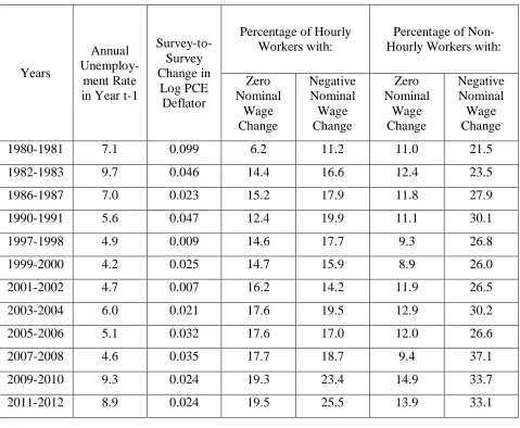
Table 1 displays men’s mean and median log real wages by year. Results are shown for
two deflators, the personal consumption expenditures (PCE) deflator from the national income
accounts (the version available in May 2014) and the CPI-U-RS version of the consumer price
3
Unweighted estimates turn out to be similar. Excluding observations with imputed wages results in higher mean and median wages, but has almost no effect on measured cyclical variation.
4
5
index.5
The first thing to note in Table 1 and Figure 1 is the stagnation of men’s real wages over
the 1979-2012 period. Real wages at the end of the period are much the same as at the
beginning. Although this is bad news for us as male workers, it is convenient for us as
researchers. With almost no secular trend, it becomes easy to discern cyclical patterns.
Both are scaled to express real wages in 2009 dollars. Figure 1 adds a visual display of
the real wage series based on the PCE deflator. The table and figure also show the annual
unemployment rate, to emphasize which years are recession years and which are expansion
years.
Like previous microdata-based studies, Table 1 and Figure 1 indicate that men’s real
wages are substantially procyclical. For example, from 1979 to 1983, when the unemployment
rate went from 5.8 to 9.6, the mean log real wage based on the PCE deflator fell from 2.906 to
2.862, a reduction of 0.044 (as also shown in Table 2, which provides a 0.005 standard error for
the estimated change between 1979 and 1983).6
What interests us most, though, is the experience of the Great Recession. The
unemployment rate, which was 4.6 in 2006 and 2007, reached 9.6 in 2010 and was still at 8.1 in
2012. Even though this run-up in the unemployment rate was even greater than that of the early
1980s, the reduction in men’s real wages was comparatively modest and gradual. The mean log
real wage based on the PCE deflator was slightly above 3.00 in 2006 and 2007, had dropped only
to 2.995 by 2010, and declined to 2.982 by 2012. Compared to the 0.044 reduction from 1979 to
1983, the 0.020 reduction from 2006 to 2012 was significantly smaller (in both the statistical and
substantive senses). Similarly, with wages deflated instead by the CPI-U-RS, the 2006-12
reduction in the mean log real wage was 0.038, as compared to the 0.057 reduction of 1979-83. With the CPI-U-RS used as an alternative
deflator, the estimated wage reduction of 0.057 is even larger. The recession of the early 1990s
was much less severe, but still was associated with a large reduction in the mean log real wage.
The recession of the early 2000s showed relatively little impact on the labor market, as reflected
in either the unemployment rate or the mean log wage.
So far we have discussed means, but there is considerable merit in looking at medians as
well. For one thing, medians are more robust to outliers. In fact, the medians stay the same
5
Other deflators, such as the GDP deflator, deliver qualitatively similar results.
6
6
regardless of whether we do or do not trim the top and bottom 1% of wage observations.
Relatedly, medians sidestep the problem of earnings codes in the CPS. Before 1996,
coded earnings observations were simply assigned the code threshold. Since 1996, a
top-coded individual has been assigned the sample mean value among all cases above the threshold
that share the individual’s gender, race, and status vis-à-vis full-time/full-year work. As a result,
our means of log real wages before and after 1996 are not altogether comparable. The medians,
however, are comparable over time because they are unaffected by the treatment of top-codes.
As can be seen in Tables 1 and 2, our medians tell much the same story as the means.
From 1979 to 1983, the median log real wage based on the PCE deflator decreased by 0.056, and
the one based on the CPI-U-RS decreased by 0.069. In contrast, from 2006 to 2012, the one
based on the PCE deflator decreased by only 0.032, and the one based on the CPI-U-RS fell by
only 0.050. The medians, like the means, indicate that real wages are considerably procyclical,
but the procyclicality of men’s real wages has been somewhat milder in the Great Recession than
in the recession of the early 1980s.
The cyclical patterns in these mean and median wage series are subject to a
countercyclical composition bias because our sample selection criterion requiring at least 100
annual hours of work disproportionately screens out low-wage workers during recessions. We
can partially correct for that bias by controlling for year-to-year changes in the demographic
composition of our samples. For example, as shown in Table 2, in addition to showing mean log
wages for each year in the 1979-83 period, we also estimate “regression-adjusted” year effects
by applying least squares (again weighting by the provided CPS sampling weights) to a
regression of individual workers’ log real wages on year dummies for 1980, 1981, 1982, and
1983 (with 1979 as the omitted reference category) and controls for years of education, a quartic
in potential work experience (age minus years of education minus 6), and race dummies.7
We perform the same exercise for the 2006-12 period. We estimate each period’s
regression separately because it is implausible that the coefficients of the control variables would As
expected, the regression-adjusted year effects show even more wage procyclicality. Whereas the
unadjusted means indicate that log real wages were 0.044 lower in 1983 than in 1979, the
adjusted 1983 year effect is 0.059 less than the 1979 effect.
7
7
come close to holding still over the entire 1979-2012 period. For example, our estimated
coefficient of education is 0.072 (with standard error 0.0006) for the 1979-1983 period, but it is
0.111 (0.0005) for 2006-2012. Whereas the unadjusted means indicate that log real wages were
0.020 lower in 2012 than in 2006, the adjusted 2012 year effect is 0.037 less than the 2006 effect.
Again, however, this wage drop in the Great Recession is significantly smaller than the wage
decrease during the early 1980s recession.
For the same reasons it was worthwhile to calculate medians along with means, it makes
sense to estimate median regressions as well as mean regressions. In the last column of Table 2,
we report the estimated year effects from applying weighted least absolute deviations to the
regression of log real wages on year dummies and control variables. The results indicate again
that men’s real wages decreased during the Great Recession, but not as much as in the recession
of the early 1980s.
In most instances, the regression adjustments indicate that accounting for observed
heterogeneity reveals greater procyclicality in real wages. Presumably, accounting for
unobserved heterogeneity would move further in the same direction. The traditional approach to
accounting for unobserved heterogeneity in the microdata-based literature is to control for
worker fixed effects by tracking the same workers over time in a panel survey. Although the
rotating panel design of the CPS makes it possible to follow a portion of one March’s sample to
the next March, the CPS is far from ideal for longitudinal analysis. The sample sizes for
March-to-March matches are almost always less than one-third of the sample sizes for the
cross-sections. Worse yet, one of the sources of the sample loss is that the CPS does not follow
residential movers, and exclusion of movers is an endogenous sample selection in a study of
wage changes. Nevertheless, as a further check on our results from repeated cross-sections, we
have analyzed year-to-year real wage growth for the subsamples of workers we can match
between adjacent March Current Population Surveys. As reported in detail in the working paper
version of our study (Elsby et al., 2013), the longitudinal results corroborate our finding from
repeated cross-sections that U.S. men’s real wages are procyclical, but somewhat less so in the
Great Recession than one might have expected from earlier recessions.
Table 3 shows mean and median log real wages by year for women, as Table 1 did for
men. And Figure 2 provides a visual display for women, as Figure 1 did for men. Where Table
8
well-known rise in women’s wages during the 1979-2012 period. All our measures suggest that,
over the period as a whole, women’s real wages rose at a rate of close to 0.10 per decade.
This upward secular trend in women’s wages makes it trickier to distill the cyclical
patterns. Nevertheless, inspection of Table 3 and Figure 2 reveals a clear tendency for women’s
real wages to rise more slowly during recessions. And in the Great Recession in particular,
women’s real wage growth appears to have stalled out completely. The relatively large effect
that the Great Recession appears to have had on women’s wages stands in contrast to its effect
for men, which was smaller than in the recessions of the early 1980s and early 1990s. But a
conclusive judgment on this will require additional years of data because a possible reading of
Figure 2 is that women’s real wage growth was starting to peter out before the Great Recession.
If the upward trend in women’s wages resumes in the years to come, the cyclical impact of the
Great Recession will appear large. If it does not resume, the stalling-out will be interpreted
instead as a change in secular trend.
Table 4 highlights the effects of the two most severe recessions on women’s wages, as
Table 2 did for men’s wages. In addition to showing the relative movements in mean and
median log wages, the table also presents regression-adjusted series that account for variation in
the samples’ education, potential experience, and race. As in Table 2 for men, these adjustments
suggest even greater procyclicality in real wages. After adjustment, there appears to be virtually
no real wage growth for women during the recession of the early 1980s, and negative growth
during the Great Recession. And again, as detailed in Elsby et al. (2013), we have replicated
these findings in a longitudinal analysis of workers matched between adjacent March surveys.
To summarize, our evidence for 1979-2012 from March Current Population Surveys
corroborates and updates the findings from earlier microdata-based studies that real wages in the
United States are substantially procyclical. For men, however, we find that real wages took a
smaller hit in the Great Recession than might have been expected from the experience of earlier
recessions. Our results for women are less clear-cut because of the confounding of cyclical and
trend variation, but a tentative impression is that women’s real wages may have taken a relatively
9
II. Nominal Wages and Inflation in the United States
Some recent discussions have suggested that the high U.S. unemployment during the
Great Recession may have been amplified by sluggish wage adjustment due to a combination of
low inflation and downward nominal wage rigidity.8
Thus, at least for men (though apparently not for women), that the Great Recession
reduced real wages less and more belatedly than in previous recessions suggests a possible role
for the inflationary environment. At the outset of the recession of the early 1980s, inflation was
unusually high, and employers could reduce real wages substantially even while granting
nominal wage increases. This was still somewhat true in the recession of the early 1990s, when
annual inflation was about 4%. But during the Great Recession, especially in 2009, the inflation
rate was lower, and substantial real wage cuts would have required nominal wage cuts.
Economists going back at least to Keynes (1936) have suggested that resistance to nominal wage
cuts can constrain the response of real wages to slack labor demand, and that this wage stickiness
might exacerbate rising unemployment during recessions.
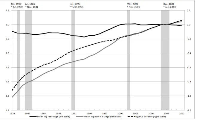
A preliminary basis for this suggestion is
illustrated in Figure 3, which decomposes the men’s mean log real wage series already shown in
Figure 1 into the difference between the mean log nominal wage and the log of the price level.
As discussed in the previous section, men’s real wages declined considerably during the
recessions of the early 1980s and early 1990s. Figure 3 shows that nominal wages grew during
those recessions, but more slowly than the price level. In the Great Recession, when men’s real
wages declined less and more belatedly than in the recessions of the early 1980s and early 1990s,
nominal wages grew very little, but so did the price level. In 2009, when the unemployment rate
was 9.3%, inflation as measured by the annual PCE deflator was virtually zero (and was slightly
negative according to the CPI-U-RS). With no decline in nominal wages that year, real wages
did not decline either. After 2009, inflation ran at about 2% a year, and the even smaller growth
in nominal wages meant that real wages underwent a modest decline.
This possibility that downward stickiness in nominal wages can impede wage
adjustments to negative labor demand shocks has led numerous researchers (for example,
8
10
McLaughlin, 1994; Card and Hyslop, 1996; Kahn, 1997; Altonji and Devereux, 1999; Dickens et
al., 2007; Elsby, 2009; and Daly et al., 2012) to examine longitudinal microdata to assess the
prevalence of nominal wage stickiness in the United States. Because it is obvious that job
changers typically experience wage changes, most of these researchers have focused on the more
interesting question of whether workers staying with the same employer appear to experience
nominal wage stickiness. What would be more interesting still would be to ascertain how many
workers lose their jobs and become unemployed because of downward stickiness in nominal
wages, but no one knows how to do that. Instead, the implicit assumption in this literature is
that, if downward rigidity in nominal wages is sufficiently common to cause a lot of job losses, it
also should be common among workers that stay employed with the same employer. In this
section, we use longitudinally matched data from Current Population Surveys to extend this
literature and update it to include the Great Recession.
Our analysis begins with the Current Population Surveys of January 1981, January 1983,
January 1987, January 1991, February 1998, February 2000, January 2002, January 2004,
January 2006, January 2008, January 2010, and January 2012. Each of these waves of the CPS
included a job tenure supplement, which enables us to determine whether a worker had been
employed for at least a year with the worker’s current main employer. We focus on such
workers in their eighth (and last) month in the CPS because workers in that “rotation group” also
were asked to report their current nominal wage rate. Using methods for longitudinal matching
recommended by Madrian and Lefgren (2000), we match these workers to their data in the CPS
one year earlier, when these workers were in their fourth month in sample.9 The fourth rotation
group is the other “outgoing” rotation group asked to report a current nominal wage rate, so we
are able to obtain an empirical distribution of year-to-year nominal wage growth of stayers for
January 1980-January 1981, January 1982-January 1983, …, January 2011-January 2012.
Fortunately, these matches include at least one year-to-year change from every recession from
the 1980s on, as well as several expansion years.10
9
In particular, we verify that longitudinal matches on identification numbers are true matches by requiring that gender and race also match and that year-to-year change in reported age is between -1 and 3.
10
11
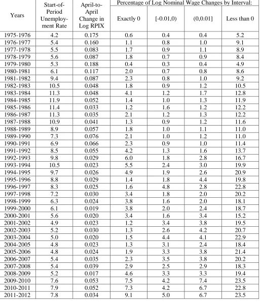
Like many previous studies, we construct histograms of the empirical distribution of
year nominal wage changes. In the interest of boosting sample size, each of our
year-to-year matched samples pools women and men between the ages of 16 and 64 in both year-to-years. We
exclude observations for which wages were imputed on account of non-response. We use the
outgoing-rotation-groups sampling weights to adjust for the Current Population Survey’s
oversampling of less populous states (though, in practice, this turns out not to affect the results
much).
For each year-to-year match, we have constructed two histograms – one for workers paid
by the hour in both years and one for workers not paid by the hour in either year. For the former,
we use the reported hourly wage rate. For the latter, we follow Card and Hyslop (1996) in using
the reported usual weekly earnings. In Card and Hyslop’s words, “In principle, we can construct
an hourly wage for non-hourly-rated workers by dividing usual weekly earnings by usual weekly
hours. However, any measurement error in reported hours will lead to excessive volatility in
imputed hourly wages.” The typical sample size for each of our histograms is about 1,000
workers. Accordingly, the typical standard error for the estimated percentage of workers with
exactly zero nominal wage change from one January or February to the next is about one
percentage point.
Each of our histograms features a thin spike at zero, which shows the percentage of the
workers that reported the exact same wage in both years. The next bin to the right of the zero
spike contains workers whose change in log nominal wage was positive but no greater than 0.02;
the next bin contains those whose change in log nominal wage was greater than 0.02 and less
than or equal to 0.04; etc. The bins to the left of zero are constructed symmetrically. To limit
the histograms to a readable scale, we pile up workers with change in log nominal wage greater
than 0.64 in the rightmost bin and those with change less than -0.34 in the leftmost bin.
Our working paper (Elsby et al., 2013) displays the entire set of histograms. For brevity,
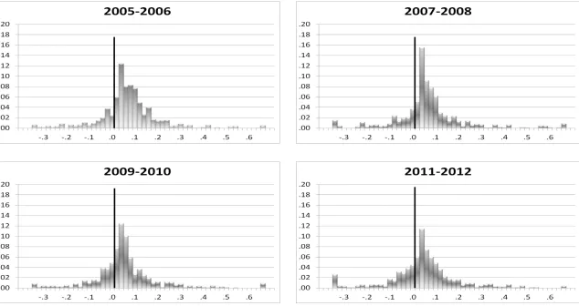
we summarize the results here in two ways. In Figure 4, we show the histograms for hourly
workers in the four most recent pairs of years. In Table 5, we present some summary statistics
for both hourly and non-hourly workers in all twelve pairs of years.
In general, our histograms display several features noted by previous authors. First, a
non-trivial fraction of workers reports nominal wage reductions in every pair of years. As shown
12
workers. While this pattern is initially suggestive of downward flexibility in nominal wages, it is
theoretically possible that the pattern is at least partly an artifact of reporting error. Workers
whose true nominal wages stayed the same or increased could be measured as experiencing
decreases if the second year’s reporting error is sufficiently negative relative to the first year’s.
Later in this paper, we will return to that possibility in light of evidence from other data sources.
Second, there is always a substantial spike at zero, which is suggestive of a degree of
nominal wage stickiness. As shown in Table 5, for each type of worker in each pair of years, a
non-trivial minority of workers ranging between 6 and 20% reports the exact same nominal wage
in both years. It is unclear a priori in which direction these estimates are biased by reporting
error. On one hand, a worker with the same true nominal wage in both years may be recorded as
changing wages if the worker misreports the wage in either year. On the other hand, a worker
with a modest wage change may round to the same number in both years and thus appear to have
zero wage change. For example, a worker whose true nominal hourly wages were $19.80 last
year and $20.30 this year may report an hourly wage of $20 in both years. When we return to
the measurement error issue in light of other evidence, we will conclude that the latter bias
dominates, so that the zero spikes in our histograms exaggerate the extent of wage stickiness.
Third, cuts and freezes in nominal wages are more prevalent when inflation is low and
labor demand is weak. Cuts and freezes were least common in 1980-81, when the inflation rate
was about 10% and unemployment was rising but had not reached the high level of 1982-83.
They were most common during the Great Recession, when unusually weak demand coincided
with low inflation. Figure 4 and Table 5, however, show that the spikes at zero wage change
were only moderately higher in the Great Recession than in the immediately preceding years. In
addition, there appears to be somewhat of an upward secular trend in the frequency of freezes,
which might be a gradually evolving response to a prolonged stretch without high inflation.11
Although we will argue that rounding error exaggerates the height of the zero spikes in
survey-based histograms, there undoubtedly is some stickiness in nominal wages. Some workers
really experience nominal wage freezes from one year to the next; many workers, including
11
13
ourselves, have their nominal wages reset only once a year; and almost no workers have their
nominal wages reset every nanosecond. The question is not whether there is any wage
stickiness. The questions are: First, how would the distribution of wage growth differ in the
absence of nominal wage stickiness? Second, whatever that difference is, what are the effects on
quantity variables like employment and unemployment? In particular, has downward nominal
wage rigidity been a major cause of the Great Recession’s unusually high unemployment?
On the first question, we reiterate that the spikes at zero nominal wage change that we
measure during the Great Recession are only moderately greater than the ones we measure for
earlier in the 2000s. Beyond that, it is remarkably difficult to identify how nominal wage growth
distributions are affected by nominal wage stickiness. As noted earlier in this section, many
excellent researchers have tackled this question before, but we are struck by how unsuccessful
they have been in reaching definitive conclusions. A particularly sophisticated effort is the
well-known study by Kahn (1997), which used substantial changes in inflation over the 1970-88
period to try to identify how nominal wage stickiness affected the distribution of wage growth
across 12 one-percentage-point bins on either side of each year’s median wage growth.
Although the approach seems conceptually promising, it delivers only two robust findings – that
there is a noticeable spike in the bin for zero nominal wage growth, and that there appears to be a
dip in the bins for 1 or 2% above zero (which, as we will discuss in the next section, also could
be a reporting effect, not a real phenomenon). All the other patterns of interest turn out to be
sensitive to functional form specification or sample selection. For example, Kahn’s results
(nicely summarized in her Table 2) indicate a tendency away from nominal wage reductions for
hourly workers, but show the opposite tendency in some specifications for non-hourly workers.
Her estimates also indicate a dip in the bin for 1% below zero for non-hourly workers, but show
no such dip for hourly workers. In the end, as is so often the case, inferring convincingly
clear-cut counterfactual distributions from observational data turns out to be beyond the reach of even
the most skillful researchers.
The second question is even harder: However much wage inertia there is, what are its
effects on employment and unemployment? Here it is helpful to make a distinction between
workers in the “primary” and “secondary” sectors of the labor market. Our histograms pertain to
workers that stayed with the same employer for at least a year. These tend to be the
14
relationships. The histograms tend to exclude workers in the secondary sector, where specific
human capital is mostly absent and labor turnover is high. There is little theoretical reason to
expect wage rigidity in the secondary sector, and Bewley’s (1999) anecdotal evidence from
extensive interviews with employers during the recession of the early 1990s corroborates the
expectation of wage flexibility in the secondary sector.
On the other hand, Bewley’s interviews also dovetail with the zero spike’s quantitative
suggestion that primary-sector employers are reluctant to cut incumbent workers’ nominal
wages. But a long history of economic analysis, dating back at least to Becker (1962), questions
whether current wages in long-term employment relationships are “allocative.” Rather, current
wages can be seen as installment payments within a longer-term compensation package. In
particular, an employer’s decision about whether to continue to employ the marginal incumbent
worker should depend on the employer’s beliefs about the present discounted value
(1) {( )/[(1 ) 1]}
1
−
=
+ −
=
∑
tT
t
t
t w r
m V
where m denotes the real value of the worker’s marginal product, w is the worker’s real wage, t
indexes time period with the current period denoted as t =1, and T is the worker’s remaining
tenure with the employer if not laid off this period. Of course, the latter is not only uncertain, but
also endogenously determined by the employer’s wage policy and future retention decisions. For
simplicity, the real interest rate r is assumed to be constant over time, and the worker’s
employment with the firm is assumed to be binary with no hours variation at the intensive
margin. Now suppose that downward rigidity in the nominal wage causes the employee’s
current real wage w1 to exceed her current real value of marginal product m1. Even so, it is in
the employer’s interest to retain the employee as long as continuing her employment is profitable
in present-value terms. Consequently, even in the face of evidence that there exists some
stickiness in current nominal wages, it does not follow that such wage stickiness necessarily
must generate inefficient job separations.
This theoretical point is buttressed by at least two pieces of empirical evidence. First is
the anecdotal evidence from Bewley’s interviews. On the question of why employers did not
save laid-off workers’ jobs by cutting their wages instead, here is Bewley’s summary (pp.
180-1): “I was surprised to learn that most managers did not believe that pay cuts would prevent
15
little or no extra work and so would barely reduce the number of excess workers.” The direct
quotations from owners and managers include these (p. 185): “If I cut pay instead of laying
people off, I would have lots of people with nothing to do.” “What do pay cuts have to do with
layoffs? A layoff is used when you don’t have sufficient work for certain skills. What would
you do with the extra help?” “Wage cuts are not an alternative to layoffs. You can’t have a lot
of people standing around doing nothing.” Whatever else one makes of these statements, they
are consistent with the proposition that downward stickiness in current nominal wages need not
be a major source of economically inefficient layoffs.
Second, returning to the Great Recession in particular, if current wages are indeed
allocative and downward nominal wage rigidity was especially binding in the Great Recession’s
low-inflation environment, one would expect the Great Recession to be characterized by an
extraordinary burst of layoffs. The behavior of the quantity side of the U.S. labor market during
the Great Recession has been documented in detail by Elsby et al. (2010). They show that, while
layoffs rose sharply during the recent downturn, the magnitude of the rise was comparable to that
seen in prior severe recessions, notably the high-inflation environment of the early 1980s (see,
for example, their Figure 9).
Instead, the most distinctive feature of the Great Recession with respect to labor
quantities has been the extraordinarily long duration of unemployment spells. Therefore,
understanding the high unemployment of the Great Recession requires understanding not only
why some employers laid off so many workers into unemployment, but also why other
employers have been so slow to hire the unemployed. Again, we find it instructive to consider
the present-value expression in equation (1), except that now we regard it as the present value of
a prospective new hire.12
Accordingly, several recent papers, such as Hall and Milgrom (2008) and Kennan (2010),
have appended various sorts of hiring-wage stickiness to the Mortensen-Pissarides (1994)
matching model in an effort to generate realistically large cyclical fluctuations in unemployment. Presumably, one major reason for employers’ reluctance to hire the
unemployed during a recession is that depressed product-market demand reduces prospective
hires’ current and near-term values of m. Even so, if current and future values of w fell
sufficiently, hiring the unemployed could become attractive to employers.
12
16
Of course, it is always possible theoretically to generate more unemployment by assuming
inflexible wages, but is the assumed inflexibility in hiring wages realistic? It is surprisingly
difficult to answer that question because most countries have no publicly available data that track
hiring wages within particular jobs within particular firms. Martins et al. (2012) use such data
from the Portuguese census of employers and find that real hiring wages in Portugal have been
quite procyclical. Their conclusion, however, acknowledges that the initial hiring wage by itself
is not a sufficient statistic for the relevant labor price. Referring again to equation (1), suppose
that the initial hiring wage w1 drops considerably in a recession, but this bargain price for labor
vaporizes quickly because, as the recession passes, the cheaply hired workers either quit (small
T) or are retained at the cost of substantial wage increases (high wt for t>1). In that case, even
a substantial drop in initial hiring wages might not raise V enough to induce primary-sector
employers to hire from the unemployed. On the other hand, as emphasized by Kudlyak (2009),
if instead workers hired at a low wage during a recession are somehow locked into a long-term
employment relationship at a persistently low wage, the labor cost relevant to employers’
recruiting decisions could be as cyclical as, or even more cyclical than, the initial hiring wage.
Therefore, assessing the practical relevance of the new theories based on inflexible hiring wages
will require more empirical work that, in the tradition of Beaudry and DiNardo (1991),
recognizes the durability of primary-sector employment relationships and studies how wage
paths in those relationships depend on current, past, and anticipated business cycle conditions.
By the same token, future theoretical research needs to analyze the nature of implicit contracts in
long-term employment relationships and consider how contracts for new workers interact with
ongoing contracts for incumbent workers. In our view, the model of Snell and Thomas (2010) is
a promising step in that direction.
In any case, we are skeptical that a theory of downward rigidity in nominal wages in
particular is the key to understanding depressed hiring during the Great Recession. We already
have noted that whatever such rigidity there is did not cause a greater upsurge in layoffs than
occurred in the high-inflation environment of the early 1980s recession. While models such as
the Snell-Thomas one recognize the possibility of spillovers from wage stickiness for incumbent
workers to stickiness in hiring wages, it is hard to imagine that nominal rigidity is more
17
appear to cause an unusually large upsurge in layoffs of incumbents, it seems implausible that it
could account for the Great Recession’s unusually long duration of unemployment spells.
To summarize, at an early stage of our research project, we were intrigued by the
possibility that the combination of downward nominal wage rigidity with low inflation might be
an important part of explaining the Great Recession’s high unemployment. With some
disappointment, we have come to feel that much of the evidence lines up poorly with that story.
Although men’s real wages seem to have taken a smaller hit in the Great Recession than in
earlier recessions, women’s wages seem to show the opposite pattern; although the histograms
show a spike at zero nominal wage change, they also show many nominal wage cuts; the zero
spike increased in the Great Recession, but not dramatically; and layoffs were not dramatically
more prevalent in the Great Recession than in earlier severe recessions.
None of this is to deny the obvious – that the Great Recession has been a terrible
economic downturn with painful consequences for many workers. Rather, we are saying that the
existence of some nominal wage stickiness is not in itself prima facie evidence that such wage
stickiness has caused an epidemic of economically inefficient choices by employers and
employees. It is conceivable that the high unemployment of the Great Recession would have
been nearly as high even in a parallel universe with absolutely flexible wages.
III. Wages in Great Britain, 1975-2012
Our analyses of real and nominal wages in Great Britain are based on the panel files from
the New Earnings Survey (NES, Office for National Statistics). These are the same data used by
Devereux and Hart (2006) to study real wage cyclicality and by Nickell and Quintini (2003) to
study nominal wage rigidity. Devereux and Hart’s sample period ends at 2001, however, and
Nickell and Quintini’s ends at 1999. We are able to update both analyses to 2012.13
Besides the substantive merit of studying wage adjustment in Great Britain in addition to
the United States, there is a methodological bonus – the NES data are superior to available U.S.
data in several ways. First, the NES sample sizes are large. The survey is based on a 1% sample
13
18
of British income taxpayers, defined by individuals whose National Insurance numbers end in a
given pair of digits. The resulting sample covers about 160,000 workers each year. Second,
since the sample frame consistently has been based on the same pair of National Insurance
number digits, the survey naturally has a panel structure. Third, the survey’s wage information is
unusually accurate. The survey is administered to employers, which are required by law to
respond to the survey. The information on earnings and work hours elicited from the employers
pertains to payroll information for a reference week in April. Because the earnings and hours
data come from payroll records, they are thought to be much more accurate than similar data
gathered from household surveys. A noteworthy limitation of the survey, however, is that it
samples from taxpayers registered in the income tax system and therefore is thought to
under-represent low-paid workers.
To provide context for our analysis, the left panel of Figure 5 displays the 1975-2012
U.K. series for the unemployment rate (as measured by the Labour Force Survey) and the
inflation rate (as measured by the change in the logarithm of the RPIX, which is based on the
Retail Price Index, but excludes mortgage interest payments). To conform to the April timing of
the NES, we use April measures for the unemployment rate and the RPIX. As the
unemployment rate shows, our sample period encompasses three recessions. Like the United
States, the United Kingdom experienced a very severe recession in the early 1980s. The
somewhat less severe episode in the early 1990s again brought the unemployment rate to double
digits. By some stroke of good fortune, the United Kingdom escaped the global contraction in
the early 2000s, but was not spared in the Great Recession. Interestingly, although the output
fall associated with the Great Recession was relatively large, the unemployment rate did not go
as high as it had in the recessions of the early 1980s and early 1990s.
As the left panel of Figure 5 also shows, the United Kingdom entered the 1980s with
even higher inflation than the United States, reaching nearly 20% on an annual basis.
Subsequently, inflation fell rapidly in the 1980s and, except for an aberration in the late 1980s
(associated with the boom at that time), remained below 5% from 1985 through to the early
stages of the current recession. Inflation did rise somewhat during the Great Recession, though,
exceeding 5% in 2010.
We will analyze real wages in part A of this section and nominal wages in part B.
19
earnings divided by hours in the reference week in April) excluding overtime. For the analysis
of real wages, we convert the nominal wage into 2012 pounds based on the April RPIX. In our
initial sample selection, we exclude individuals who reported wages for more than one job in the
reference week, who lost pay due to absence in that week, or who were younger than 16 or older
than 64, and then we trim the remaining sample for each year by excluding the cases with the top
and bottom 1% of wages.
A. Real wages
Following our U.S. analysis of real wages, we further restrict the sample to workers
between the ages of 25 and 59.14
Our main analysis of U.S. real wages used repeated cross-sections from the March CPS
that measured wages with average hourly earnings over the entire preceding calendar year. We
also referred to longitudinal results based on March-to-March matches, but with some
reservation on account of imperfections in the CPS as a source of longitudinal data, especially its
failure to follow residential movers. Somewhat in parallel, we will begin by analyzing repeated
cross-sections from the NES, but with a caveat. Because the NES measures wages only for those
working in the reference week in April, it seems potentially subject to more severe composition
bias than the March CPS. Fortunately, however, the NES is an excellent source of longitudinal
data, so we will proceed to longitudinal analyses that hold composition constant by following the
same workers from one April to the next.
The resulting sample of men is typically about 60,000 per year.
The women’s sample starts at more than 30,000 in 1975 and exceeds 60,000 in the later years of
the sample period.
Starting with the repeated cross-sections, Table 7 in Elsby et al. (2013) shows mean log
real wages by year separately for men and women. Here we display both series visually in the
right panel of Figure 5. In Great Britain, as in the United States, the upward trend in women’s
wages is dramatic. But whereas men’s wages stagnated in the United States, they have risen
considerably in Great Britain, though not nearly as much as women’s.
The cyclical patterns for men and women look similar, so we will discuss them together.
The most striking cyclical setback to real wages occurred during the Great Recession. From
14
20
2008 to 2012, as the unemployment rate went from 5.2 to 8.1, men’s real wages declined by
about 14 log points, and women’s declined by about 8. Viewed against the backdrop of the
upward secular trends in real wages, these reductions look all the more striking. The only other
prominent reduction in real wages during our sample period occurred in the non-recession year
of 1977. The story behind this episode appears to be related to incomes policies negotiated
between the British government and the trade unions at that time. The agreement placed an
upper bound on increases in nominal wages for that year, presumably in an attempt to curb
inflation by stemming wage inflation. Despite this, price inflation remained very high, and so
workers experienced real wage cuts.
Turning to the other recessions, during the early 1980s, when the unemployment rate rose
to almost 12% and inflation was even higher than in the United States, real wage growth hardly
slowed at all. The recession of the early 1990s was accompanied by a more noticeable slowing
of real wage growth, but nothing like the reduction during the Great Recession. Thus, the British
variation in wage cyclicality across recessions is more or less the opposite of what we measured
for U.S. men in Section II. This poses still another challenge to simple stories about the
interaction of downward nominal wage rigidity and the inflationary environment. In Great
Britain, real wages took a much bigger hit in the Great Recession than in the early 1980s even
though the early 1980s were a period of much higher inflation.
All of this, however, is based on wage measures from repeated cross-sections for a
reference week in April. The U.S. evidence indicates that such measures could be subject to a
substantial countercyclical composition bias, so we follow Devereux and Hart (2006) in using
the longitudinal nature of the NES to hold worker composition constant by following the same
workers from one April to the next. This longitudinal matching loses some workers not
employed in one reference week or the other, but the sample sizes are still large. The men’s
sample size per year is usually over 50,000. The women’s sample size starts at over 20,000 in
1975-76 and reaches over 60,000 towards the end of our sample period.
Table 8 in Elsby et al. (2013) shows mean year-to-year change in log real wages by
gender for each pair of years from 1975-76 to 2011-12. Here we plot this longitudinally based
series for each gender in Figure 6, along with the first difference of the cross-sectional mean log
wage series previously shown in the right panel of Figure 5. Figure 6 vividly depicts two
21
encompasses life-cycle wage growth. But second, the cyclical patterns for the longitudinal series
and the series from repeated cross-sections are remarkably similar. Although composition bias
repeatedly has been found to be an important issue for measuring wage cyclicality in the United
States, it appears to matter much less for Great Britain.15
We already have noted that this pattern cannot be explained by changes in the
inflationary environment, which go the “wrong” way. So what does account for the increasing
procyclicality of British real wages? One possibility is that declining unionization has led to
more flexible wages. Setting aside the puzzle of why the same trend has not led to greater wage
flexibility in the United States as well, we have pursued the British evidence on this idea by
redoing Figure 6 disaggregated by union status. Figure 10 in Elsby et al. (2013) shows mean
year-to-year change in log real wages by gender separately for those who were in jobs covered
by union agreements in both years and those who were in non-union jobs in both years. Those
plots for union and non-union workers are strikingly similar to each other, and to the aggregate
plots in Figure 6. Thus, although declining unionization could be part of the story, it cannot be
nearly all of it. Even after controlling for union status, the procyclicality of real wages remains
much stronger in the Great Recession than in earlier recessions.
Thus, we continue to find that real
wage growth in Great Britain hardly slowed at all in the early 1980s, slowed more in the early
1990s, and went negative in the Great Recession.
B. Nominal wages
The relative accuracy of the payroll-based NES wage data is especially valuable in the
analysis of year-to-year changes in nominal wages. It will be instructive here to begin by
reviewing two previous British studies of nominal wage rigidity. Smith (2000) used the 1991-96
waves of the British Household Panel Study (BHPS) to retrace the steps of the U.S. literature
described in our Section II. Whereas most U.S. researchers have attempted to restrict their
samples to workers staying with the same employer, Smith further restricted to workers who
reported staying in the same job with the same employer. If anything, one would expect that
difference to lead to a higher frequency of zero nominal wage change. Her initial results turned
out to be fairly similar to those from U.S. household surveys for the same period – she found that
15
22
9% of stayers experienced zero nominal wage change from one year to the next, and that 23%
experienced nominal wage reductions.
But then she exploited a remarkable feature of the BHPS data – respondents were told
they could consult their pay slips when answering the wage questions, and the survey recorded
who did so. When Smith restricted her sample to those who did check their pay slips in both
years, the proportion with zero nominal wage change fell to 5.6%. As we mentioned in Section
II, it is ex ante unclear in which direction reporting error would bias the estimation of the spike at
zero nominal wage change. Purely classical measurement error would bias the estimation
downward, but rounding error could go the other way. For example, a worker whose hourly
wage was £11.93 last year and is £12.17 this year might round to £12 in both years and get coded
as experiencing zero change. Smith’s results suggest that, on net, nominal wage change
distributions from household surveys overestimate the proportion of stayers with zero nominal
wage change. Unsurprisingly, she also found that, among the respondents who did check their
pay slips, the proportion reporting nominal wage reductions was somewhat smaller. But it was
still quite substantial, at almost 18%. In combination, Smith took these results as showing that
nominal wages are considerably more flexible than economists had believed. To quote her
striking summary, “Some of the results in this paper may seem difficult to believe – the quite
common occurrence of nominal pay cuts, for example. It may well be that the difficulty in
believing them stems not from the weight of contradictory evidence, but rather from
conventional wisdom that has survived because of the previous lack of evidence either way.”
Smith’s study was following by Nickell and Quintini’s (2003) study based on the NES
data for 1975-99. Like Smith, Nickell and Quintini focused on workers staying in the same job
with the same employer. Nickell and Quintini began by comparing their 1991-96 nominal wage
change measures, based on employers’ payroll-based reporting, to Smith’s household survey
measures for the respondents who consulted their pay slips. The results from the two sources
line up quite closely with each other. More generally, over their full 1975-99 sample period,
Nickell and Quintini found that there was regularly a noticeable spike at zero nominal wage
change, but that it was much smaller than usually found in household surveys. In most years, the
proportion of stayers with zero nominal wage change was less than 3%, with the highest
proportion being 7.1% in 1992-93. And despite the presumed accuracy of the employers’ wage
23
substantial, ranging from a low of 5% in 1979-80 (when the inflation rate was close to 20%) to a
high of 22% in 1996-97. Nickell and Quintini concluded, “Despite the substantial numbers of
individuals whose nominal wages fall from one year to the next, we find that there is evidence of
some rigidity at zero nominal wage change. While the effect is statistically significant, the
macroeconomic impact of the distortion is very modest.”
Our analysis of the NES data updates Nickell and Quintini’s analysis to 2012. As in our
U.S. analysis of nominal wages in Section II, we pool women and men between the ages of 16
and 64. Unlike in our U.S. analysis, we pool hourly and non-hourly workers, who are not
distinguished in the NES data. Because our analysis of year-to-year nominal wage changes is
restricted to workers staying in the same job with the same employer, our sample sizes become
somewhat smaller than in our longitudinal analysis of real wages in the NES. With women and
men combined, our sample size starts at almost 60,000 for 1975-76 and rises to over 100,000 by
the end of our sample period.
In Elsby et al. (2013), we present a complete set of histograms of job stayers’
year-to-year nominal wage growth for each pair of year-to-years from 1975-76 on. Here we summarize by
showing the histograms for the six most recent pairs of years in Figure 7, along with summary
statistics for all years in Table 6. The histograms are laid out similarly to our U.S. ones except
that Figure 7 combines hourly and non-hourly workers. Because the spikes at zero are less
prominent in the British data, we highlight them in dark blocks instead of thin lines.
Four patterns stand out in the histograms and table. First, like Nickell and Quintini, we
find relatively small spikes at zero nominal wage change, ranging from a low of 0.4% in 1979-80
to a high of 9.1% in 2011-12. In most years, the spike is less than 3%. That the zero spikes are
so much smaller in the British payroll-based data than in the U.S. household survey data suggests
a possibility that the larger U.S. spikes might be at least partly an artifact of rounding error.
Second, we replicate and update the finding of substantial proportions of British job
stayers experiencing negative nominal wage changes. Our estimates range from a low of 4.9%
in 1979-80 to a high of 23.5% in 2009-10 and 2011-12. From 1993-94 on (when the inflation
rate typically has been about 3%), the proportion experiencing nominal wage cuts regularly has
run in the neighborhood of 20%.16
16
Furthermore, these nominal wage cuts are remarkably pervasive across sub-groups of workers/jobs. For example, in 2011-12, when the overall proportion of job stayers experiencing cuts was 23.5%, the proportions were 22% in
24
struck by the wage flexibility indicated in the frequency of nominal wage cuts as well as the
infrequency of nominal wage freezes. Some U.S. writers, such as Altonji and Devereux (1999),
have conjectured that the substantial fraction of U.S. job stayers reporting nominal wage
reductions is an artifact of response error in household surveys. The payroll-based British data,
however, also show many nominal wage cuts.
Third, as in previous research for both Great Britain and the United States, the fractions
of job stayers with zero and negative nominal wage changes vary over time with respect to
inflation and business cycle conditions in the ways that one would expect. In the first few years
of our British sample period, when inflation was particularly high, the fractions with zero and
negative nominal wage changes were particularly low. In the last three years of the sample
period, when the Great Recession was at its worst and inflation was moderate, the fractions with
zero and negative nominal wage changes were higher than usual.
Fourth, some of the household-survey-based U.S. literature, such as Kahn (1997), has
noted some evidence for dips in the distribution of nominal wage change in the bins immediately
surrounding zero, and has interpreted those dips as possibly reflecting menu costs in wage
setting. Such dips are not particularly apparent in our histograms from the British payroll-based
data. And, as shown in Table 6, the percentages of job stayers with positive and negative log
nominal wage changes no larger than 0.01 are non-trivial, reaching a combined share of 11-12%
in the last three years of our sample period. This leads us to wonder whether rounding error in
U.S. household surveys has not only exaggerated the spike at zero nominal wage change, but has
done so by reducing the reporting of small non-zero nominal wage changes, thus creating the
appearance of dips around zero in the histograms.17
Payroll-based longitudinal hourly wage data for the United States would be invaluable for
exploring our conjectures about how rounding and other measurement error may distort U.S.
survey-based measures of nominal wage change. Fortuitously, Kurmann et al. (2014) recently
the private sector and 26% in the public sector; 27% for union workers and 22% for non-union workers; at least 20% for every single-digit occupation; and 32% for workers that received incentive pay in either 2011 or 2012 and 22% for workers that did not.
17
25
discovered that, for three U.S. states (Minnesota, Rhode Island, and Washington), the
Longitudinal Employer-Household Dynamics data include payroll-based reports of workers’
quarterly hours as well as earnings. At our request, Kurmann et al. graciously have constructed
histograms of year-to-year changes in nominal average hourly earnings from quarters of 2010 to
the corresponding quarters of 2011. These pertain to workers who stayed with the same
employer from the fourth quarter of 2009 to the first quarter of 2012. For comparison, recall that
the CPS results in our Table 5 show that, in 2009-10 and 2011-12, the percentages of stayers
with zero nominal wage change were over 19% for hourly workers and almost 15% for
non-hourly workers, while the percentages with nominal cuts were 23-26% for non-hourly workers and
33-34% for non-hourly workers. The payroll-based results from Kurmann et al. show only 4%
with zero nominal wage change, but 24% with nominal wage cuts of at least half of 1%. These
payroll-based results, like our British results, lead us to suspect that downward nominal wage
rigidity may be less binding than is often supposed.18
IV. Summary and Discussion
Our analyses of both U.S. and British data replicate and update the finding of previous
microdata-based studies that, by and large, real wages are substantially procyclical. The degree
of real wage cyclicality, however, varies over time and place. Our analysis of March Current
Population Survey data for the United States suggests that real wages took large hits in the
recessions of the early 1980s and 1990s, but that men’s real wages were somewhat less affected
in the Great Recession. Because of difficulty in separating cyclical effects from secular trends,
the picture for U.S. women is less clear, but a tentative impression is that the Great Recession’s
impact on U.S. women’s real wages was particularly adverse. Our analysis of New Earnings
Survey data for Great Britain also finds differences across recessions, with practically an
opposite pattern to that for U.S. men. In Great Britain, real wages were not much affected by the
severe recession of the early 1980s, displayed slowed growth in the severe recession of the early
1990s, and were affected very negatively by the Great Recession. The between-country
18
26
difference in the evolution of real wage cyclicality over our sample period is all the more striking
given that both countries experienced reductions in inflation and unionization.
Motivated by the oft-stated hypothesis that downward nominal wage rigidity is an
important contributor to cyclical employment and unemployment fluctuations, we also have used
the CPS and NES data to replicate and update the literature that documents the distribution of job
stayers’ year-to-year nominal wage changes. Like previous studies of U.S. household surveys,
our CPS analysis finds a substantial minority of stayers reporting the exact same nominal wage
from one year to the next (seemingly indicating a degree of wage rigidity), but also a substantial
minority reporting nominal wage reductions (seemingly indicating a degree of wage flexibility).
As previous writers have noted, both findings may be distorted by reporting error. This makes
the presumably more accurate NES wage data, reported by employers from payroll records, of
particularly high interest. These data show a much lower frequency of zero year-to-year nominal
wage change, but they show a surprisingly high frequency of nominal wage reductions. Like the
authors of previous British studies of nominal wage change, we are struck by the apparent
flexibility of British wages. Preliminary payroll-based evidence for the United States from the
Longitudinal Employer-Household Dynamics data suggests that U.S. wages also may be less
rigid than is often supposed.
However much wage stickiness there is, does it have important effects on employment
and unemployment? In particular, did its interaction with an environment of very low inflation
contribute to the large upsurge of U.S. unemployment in the Great Recession? At an early stage
of our project, we thought this story was suggested by the sluggish response of men’s real wages
to that downturn. But, while there may be something to the story, it lines up poorly with many
other empirical patterns. Why did the Great Recession appear to have a particularly large effect
on U.S. women’s real wages? Why didn’t the prevalence of zero nominal wage change rise
more precipitously during the Great Recession? As discussed in Section II, there are theoretical
reasons to question whether wage stickiness has major “allocative” effects, and empirically, if it
does, one would expect the Great Recession to have featured an extraordinarily large upsurge in
layoffs. Layoffs did indeed surge upwards, but similarly to how they did in previous severe
recessions, including the high-inflation environment of the early 1980s. The more distinctive
aspect of the U.S. labor market’s response to the Great Recession has been the extraordinary