Munich Personal RePEc Archive
Micro-level Rigidity vs. Macro-level
Flexibility: Lessons from Finland
Böckerman, Petri and Laaksonen, Seppo and Vainiomäki,
Jari
6 May 2009
Online at
https://mpra.ub.uni-muenchen.de/15061/
T A M P E R E E C O N O M I C W O R K I N G P A P E R S
N E T S E R I E S
MICRO-LEVEL RIGIDITY VS. MACRO-LEVEL FLEXIBILITY: LESSONS FROM FINLAND
Petri Böckerman, Seppo Laaksonen, Jari Vainiomäki
Working Paper 72 May 2009
http://tampub.uta.fi/econet/wp72-2009.pdf
DEPARTMENT OF ECONOMICS AND ACCOUNTING
FI-33014 UNIVERSITY OF TAMPERE, FINLAND
Micro-level Rigidity vs. Macro-level Flexibility: Lessons from Finland
Petri Böckerman*, Seppo Laaksonen** and Jari Vainiomäki***
* Labour Institute for Economic Research and University of Tampere. E-mail:
** University of Helsinki and University of Tampere. E-mail: [email protected]
*** University of Tampere. E-mail: [email protected]
Abstract
This paper explores the wage flexibility in Finland. The study covers the private sector
workers by using three data sets from the payroll records of employers’ associations. The
data span the period 1985-2001. The results reveal that there has been macroeconomic
flexibility in the labour market. Average real wages declined during the early 1990’s
depression and a large proportion of workers experienced real wage cuts. However, the
evidence based on individual-level wage change distributions shows that especially real
wages are rigid. In particular, individual-level wage changes have regained the high levels
of real rigidity during the late 1990s that prevailed in the 1980s, despite the continued high
(but declining) level of unemployment.
Keywords: Wage flexibility; wage rigidity; wage cuts
Correspondence:
Jari Vainiomäki
Department of Economics
FI-33014 UNIVERSITY OF TAMPERE
FINLAND
I. Introduction
This paper evaluates the wage adjustment in Finland by using data from the payroll records
of employers’ associations.1 The Finnish case provides particularly interesting environment
to examine the wage flexibility for three reasons. First, there was an unprecedented collapse
in aggregate economic activity during the early 1990s. Output fell by 14% in the years
1990-1993. The unemployment rate increased in three years (1991-1993) to almost 20%
from an average around 5% during the 1980s. Thus, Finland suffered its worst depression
of the twentieth century not in the 1930s but in the early 1990s (e.g. Honkapohja and
Koskela 1999; Böckerman and Kiander 2002; Koskela and Uusitalo 2006; Gorodnichenko
et al. 2009). It is possible that this shock to unemployment caused changes in the way
labour markets work and affected the strictness of constraints to downward rigidity of
wages.
Second, Finland has been a high-inflation country, where the rapid rate of inflation was
compensated by the frequent devaluations of currency to regain competitiveness in export
sectors. This traditional pattern of macro-level adjustment turned around when the Bank of
Finland adopted inflation targeting after the depression of the early 1990s and the country
joined to the third stage of Economic and Monetary Union in 1999. In February 1993 the
Bank of Finland adopted a target rate of 2% per annum for the core inflation rate to be
attained by 1995. The same target was upheld by the European Central Bank. The target
was low given the inflation history of the three previous decades. The average inflation in
Third, the structure of wage bargaining involves a high degree of coordination between
both unions and employers, with a framework agreement being determined centrally on a
one- or two-year basis, followed by union-level bargains (e.g. Vartiainen 1998). Hence,
collective bargaining dominates wage formation and the coverage of collective bargains is
roughly 95% of all workers, one of the highest rates in the OECD (e.g. Layard and Nickell
1999). As one outcome of the binding collective agreements, wage compression is high.
Despite discussions and pressures for changes in the institutions, the wage setting practices
can be described as stable over the period of analysis (1985-2001).2
This article is structured as follows. Section 2 provides descriptive evidence. Section 3
reports results on the incidence of wage cuts. Section 4 analyses the micro-level rigidity of
wages and Section 5 focuses on macro-economic adjustment. The last section concludes.
II. Wage Changes
We use three separate data sets for the private sector workers obtained from the payroll
records of employers’ associations for the period 1985-2001.3 The observed wage change
distributions are presented in Figs. 1-6. The distributions are centered around the contract
wage change or actual inflation each year and then averaged over the years. The figures
include also a symmetrical distribution around the median bin of the averaged distribution.
For the contract wage this median bin is always the zero bin. For inflation the median bin is
are the percentage wage changes implied by the contracts signed in each bargaining round
as reported in Marjanen (2002) and they can be different for the three sectors.
Figs. 1-6 around here
In all sectors there is a peak in the distribution at the level of nominal wage increase
stipulated in the collective agreements. The share of observations below the contact wage
rise is substantially less than in a symmetric distribution. Hence, there is a cut-off in the
distribution at the contract wage rise or just below it, and missing mass below that point.
Compared to a similar distribution centered around inflation it is obvious that the contract
wage rise determines the concentration of observations more than inflation. For inflation
centered distribution the median bin is above the inflation bin, and there are excess
observations several percentage points below the inflation rate (for the blue-collar workers
this excess is smaller). Thus, the shape of wage change distribution depends mainly on
general wage increase that is agreed upon in the collective agreements, and it might be
dubbed as contract wage rigidity. Alternatively, these features indicate that the centralized
bargaining institutions are the means that effectively produce real wage rigidity in wage
setting. These same institutions may, however, also be means to secure concerted
macro-level wage moderation, as discussed below.
There is not much evidence for nominal wage rigidity in annual distributions since there are
no spikes at zero wage change for manual workers, and only very small spikes for
non-manual and service sector workers.4 However, during the depression years in 1992 and
prevailing contracts. This centralized wage freeze created a large increase of zero nominal
wage changes in these years (more prominent for non-manual manufacturing workers and
service sector workers; for the service sector this freeze also continued to 1994). The
distributions for the non-manual manufacturing and service sector workers are highly
asymmetric below zero nominal wage change suggesting the presence of downward
nominal wage rigidity. However, this lack of nominal wage cuts can also be induced by real
rigidity. The small zero spikes suggest that this is most likely the case.
There have been four industry-based contracts (1988, 1994, 1995 and 2000). The
distributions in these years have not been very different from the histograms in surrounding
years with centralized contracts, but there is some tendency that the support of the mode of
wage changes is wider. This is consistent with somewhat more variation across industries
in the ‘average’ wage change in the years of industry-level contracts. For both manual and
non-manual manufacturing workers it is notable that after the depression the distributions
are different from those before the depression in the sense that the distributions have
become more concentrated during the late 1990s. The reason is that the Income Policy
Agreements have been more comprehensive during the late 1990s as a consequence of
macroeconomic difficulties, which has lead to the compression of wage changes around the
level of centralized agreements.
Along with the general rise, the collective agreements also include low-wage or female
allowances with a purpose of increasing the wages for some groups more than by the
general rise. In addition, a mixed pay rise formula (X% or Y euros at minimum) is often
annual wage changes at the individual level in current year on wage levels two years
earlier, because measurement error would produce the negative effect when using wage
levels one year earlier. We include a full set of year and industry indicators to focus on
wage compression across individuals within industries. There is evidence for a negative
relationship that supports the prevalence of solidaristic wage setting in all sectors (Table 1).
Hence, low-wage workers tend to get higher wage rises within industries. The effect is
much smaller for the non-manual manufacturing workers, because individual-level wage
bargaining is more important among them. It is also possible that the average wage level of
non-manuals is so high that the solidarity aspects do not cover them. It is likely that wage
compression biases real rigidity measures downwards, because some individuals are raised
above the real rigidity zone, rather than to the zone, in the wage change distribution.
Table 1 around here
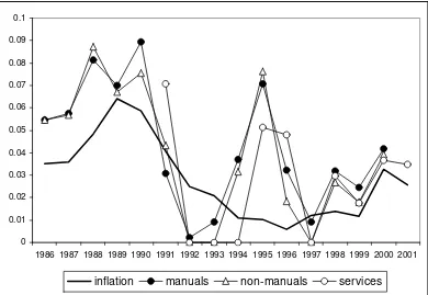
The median wage change has been strongly pro-cyclical in all sectors, and the development
of the medians over time reflects strongly the evolution of inflation (Fig. 7). Fluctuations in
the medians have also been in other respects largely similar across sectors. This is not a
great surprise, because the period is dominated by collective agreements that have produced
quite similar real wage rises across sectors, based on the average rate of productivity
growth in the economy. This is often referred to as the “wage norm”. The median worker
experienced real wage declines during the early 1990s. This contributed to a decline in the
labour share of the total income (e.g. Sauramo 2004; Kyyrä and Maliranta 2008). Real
wage increases of the median worker have also been smaller in the late 1990s compared to
Fig. 7 around here
III. Wage Cuts
It is a general presumption that centralized collective bargaining leads to compression in
both wage levels and wage changes. There is evidence for this in Finland, but there is still
considerable heterogeneity in wage changes. One indication of this is the existence of
nominal wage cuts and the differences in their incidence across sectors. For non-manual
workers in manufacturing and for the service sector workers, nominal wage cuts are rather
rare, in spite of the depression, with annual incidence of nominal wage cuts in the range
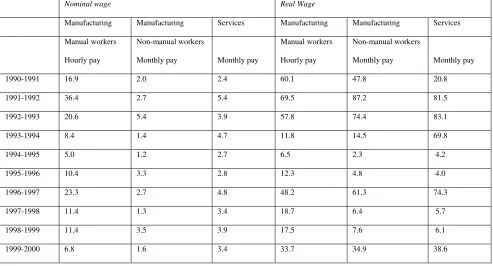
from 1 to 5 per cent (Table 2). In contrast, nominal wage cuts are much more frequent for
manual workers in the manufacturing sector, the incidence reaching 36 per cent in
1991-1992, and above 20 per cent in 1992-1993 and 1996-1997. There is also evidence that
during the depression years downward wage adjustment started earlier for manual workers
and continued longer in the service sector compared to non-manual workers.
Table 2 around here
The share of workers experiencing real wage cuts behaves remarkably similarly across
sectors, being very high (60-80%) in 1991-1993. This pattern emerges from a large number
of nominal wage increases that lie between zero and the inflation rate. This holds especially
for the non-manual and service sector workers, which explains the larger difference
moderation with the positive inflation rate during the depression made it possible to
implement real wage cuts for a large share of workers without implementing aggregate
nominal wage cuts by the collective agreements. Hence, centralized bargaining allowed for
at least some downward adjustment of real wages.5 The brief economic slowdown that
started in 1996 provides corroborating evidence for this. The bargaining system responded
to this slowdown by postponing wage rises in 1997, which is shown in the substantial
number of real wage cuts from 1996 to 1997.
The estimates from probit models can be used to evaluate the factors that have contributed
to wage cuts. The models reported in detail in Böckerman et al. (2007) include individual
characteristics (such as gender, age and working hours) and employer characteristics (such
as plant size and industry) as explanatory variables for the probability of the individual
worker experiencing a wage cut. The results show that full-time workers have a lower
likelihood of nominal and real wage decline. The service sector workers that work less than
30 hours weekly are around 4 per cent more likely to experience a nominal wage cut. The
effect is even larger for real wage reductions, which are around 9 per cent more likely for
part-time workers compared with full-time workers. For manuals and non-manuals in
manufacturing these effects are in the range of 1-3 per cent. The pattern is consistent with
the efficiency-wage explanation and the fairness standards as an obstacle to wage cuts
(Bewley 2007). Full-time workers are more important for the productivity of a firm
compared with the part-time workers and hence they have a stronger bargaining position to
fairness standards can also be tighter for the full-time insiders because of stronger
attachment with the firm.
Wage cuts are also more common in small plants. Depending on the sector, real wage cuts
are around 5-8 per cent more likely in small firms compared with large firms. For nominal
wage cuts this firm size effect is about 1-5 per cent. This result is in disagreement with
fairness as an obstacle to wage cuts. Fairness standards should be stricter in small plants,
because there are more repeated personal interactions between the employer and workers.
However, the size of a plant can matter for other reasons. It is possible that the effective
bargaining power of unions is weaker in small plants. Thus, unions are less able to resist
wage cuts in small plants that concern firm-specific wage components that do not
compromise the minimum standards stipulated in the collective agreements. Another
explanation is that greater loyalty in small plants between the workforce and the employer
can make it easier to cut wages in order to save jobs.
IV. Micro-level Rigidity
Dickens et al. (2007) present the method used for the estimation of wage rigidities in the
International Wage Flexibility Project (IWFP), and discuss its features. We use the protocol
developed in IWFP to measure nominal and real rigidities in wage setting. We concentrate
on the results based on the estimated (‘true’) wage change distribution that is corrected for
measurement errors in the data, rather than on the observed distribution.6 Generalized
change histograms. The method uses the fraction of observations in each cell of the wage
change histogram as the moments. The model assumes that, in the absence of rigidity, log
wage changes have a symmetric two-sided Weibull distribution, which is referred to as the
notional wage change distribution.7 Hence, in the absence of wage rigidities, the mean
wage change equals the median wage change. Therefore, all deviations from the symmetry
are caused by nominal and real wage rigidities. The measures are proportions of workers
that are actually subject to particular type of rigidity of those workers that are potentially
subject to the rigidity considered.8 The measures for wage rigidities vary between 0 and 1.
A value of 0 indicates perfect flexibility (no one is subject to rigidity) and 1 indicates
perfect rigidity (all workers potentially subject to rigidity are affected by it). The definition
of nominal wage rigidity is the fraction of workers who are not affected by downward real
wage rigidity, but who are affected by downward nominal wage rigidity. Thus, there is no a
priori reason for the measures of nominal and real rigidity to be negatively correlated.
We describe the results for the amount of rigidities as average values over several years,
because there have been substantial fluctuations in the measures from year to year. One
reason for the fluctuations is that it may be difficult to distinguish the effect of real wage
rigidity from the effects of collective bargaining on wage determination. Centralized wage
bargains set a floor for wage changes while allowing decentralized firm-level changes
above the floor, often called “wage drift”. The spike will then reflect the negotiated
minimum real wage change rather than the expected rate of inflation only. The protocol
restricts the expected rate of inflation to fall within reasonable bounds. Then owing to wage
drift, it is possible to estimate considerable real wage rigidity in years when the floor falls
range. Another reason is that it may be difficult to separate nominal and real wage rigidity
from each other during the years of very low inflation, i.e. during most of the late 1990s.
However, this distinction is less relevant when inflation is very low, because the effects of
nominal and real rigidities on wages are essentially the same.
We use three periods; the late 1980s (1986-1990), the early 1990’s depression years
(1991-1993/1992-1994), and the late 1990s (1994-2000/1995-2001). The results show that the
amount of nominal rigidity has been quite low in all sectors, but it rose considerably during
the depression (Table 3, Panel A). This reflects the nominal wage freeze implemented by
the collective agreements during the depression. The level of nominal rigidities was highest
in the service sector, and smallest in the manual manufacturing sector. In contrast, averages
of real rigidities reveal that the amount of real rigidities in wage changes has been smallest
during the depression (Table 3, Panel B). The level of real rigidities was lowest in manual
manufacturing and service sectors during this period. The amount of real rigidities has been
highest for non-manual manufacturing workers in the late 1980s and the late 1990s. It is
also notable that in the late 1990s the level of real rigidity has increased back to the late
1980’s levels, despite much higher level of unemployment during the late 1990s. On the
other hand, this pattern over time in real rigidity and unemployment makes it difficult to
argue that real wage rigidities are the direct cause of unemployment.
Table 3 around here
All in all, there has been a great deal of either real or nominal rigidities in all sectors in
during the depression. On the other hand, nominal rigidity increased and therefore formed
the ultimate limit to downward wage flexibility.
V. Macro-level Flexibility
To analyse the real consequences of downward nominal wage rigidity and inflation Nickell
and Quintini (2003) regress the share of negative real wage change on the inflation rate.
The control variables include the median of real wage changes and the dispersion of real
wage changes. Their results using UK New Earnings Survey over the period 1976-1999
show that an increase in the rate of inflation produces an increase in the share of workers
that experience negative real wage change. This result implies that downward nominal
rigidity and low inflation together prevent the downward adjustment in real wages.
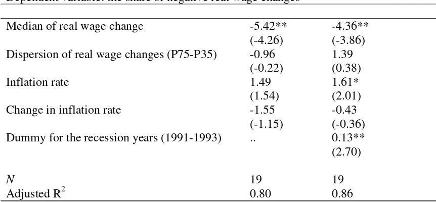
We estimate Nickell and Quintini type regressions for manual manufacturing workers.9 The
baseline model shows that the rate of inflation is not statistically significant in explaining
the share of workers that have experienced negative real wage changes (Table 4, Column
1). This is not surprising, because the share of negative real wage changes was particularly
high in manufacturing during the depression when inflation was declining (Table 2). Hence,
the result could be an anomaly related to the depression and associated disinflation. When
we include an indicator for the years 1991-1993 the relationship between inflation and the
share of workers that experience negative real wage changes is positive and statistically
significant at 10% level (Table 4, Column 2). The quantitative magnitude of the impact is
about twice as large as the one reported by Nickell and Quintini (2003) for the UK. This
target, but it suggests that lower inflation (target) together with downward nominal wage
rigidity have had some real wage effects.
Table 4 around here
As a further look at the macroeconomic flexibility of wage setting to economic conditions
we estimate simple Phillips curves or wage equations. (Pehkonen 1999 provides earlier
estimates.) That is, we regress the average changes in nominal wages on unemployment,
productivity growth and expected inflation. We also use these regressions to evaluate the
idea that downward rigidity of wages makes the adjustment of wages to economic
conditions less flexible. Since downward wage rigidities mean that wage change
distributions become asymmetric by shifting the negative nominal and real wage changes
upward in the distribution, it means that the average wage change is higher with rigidities
than without them. If the average wage change responds negatively to unemployment, the
wage changes will become more constrained from below by rigidities when unemployment
is higher. This implies that the response of average wage change to unemployment is
smaller than without rigidities. We look at this effect by using the mean wage change from
the estimated notional wage change distribution as the dependent variable in addition to the
observed mean wage change. As noted earlier, the notional wage change distribution is a
counterfactual distribution that would appear in the absence of rigidities for wage changes.
It is symmetric around the mean change. If downward rigidities in wages prevent the
adjustment of wages to economic conditions, the unemployment coefficient should be
distribution, compared to the coefficient for the observed mean. The estimated mean of
notional wage changes and expected inflation originate from the protocol of IWFP.
We report the results from the data in which we have pooled all sectors in Table 5. The
lagged productivity growth is more significant than the current one, so we use it. The past
observed productivity growth is probably taken into account in wage negotiations rather
than the expected productivity growth during the contract period. For the service sector
productivity growth is lagged two years as it seemed to work best. This indicates that the
wage setting in services follows that of manufacturing sector’s by one year lag. The most
important finding is that a significant negative relationship between wage growth and
unemployment emerges. The effect of unemployment on the observed mean wage change
is -0.4 in Column 1. The estimate is very close to what has been reported for Finland earlier
(Uusitalo 2005). We also find that the effect of unemployment on the estimated mean wage
change in Column 2 is almost the same as the one of the observed mean wage change. This
is in contrast to the idea that the responsiveness of wages to unemployment is prohibited by
downward wage rigidities. The observed wage changes seem to adjust to unemployment in
the same way as the notional wage changes that are not affected by rigidities.10
Productivity growth affects wage changes positively, with a coefficient of 0.5 in both of the
models. The industry-level bargains increase wage growth by 2 percentage points compared
to years with centralized bargains, a result consistent with the earlier evidence (Uusitalo
005).
able 5 around here 2
The measures for wage sweep up capture the extra amount of wage growth that arises
because of downward wage rigidity. They can be included as additional variables in
explaining unemployment to learn about the consequences of micro-level rigidities (see
Dickens et al. 2007). The average wage sweep up can be interpreted as the increase in
average labour costs due to downward wage rigidity. If firms are sensitive to unit labour
costs, then a higher average wage sweep up should be associated with lower employment or
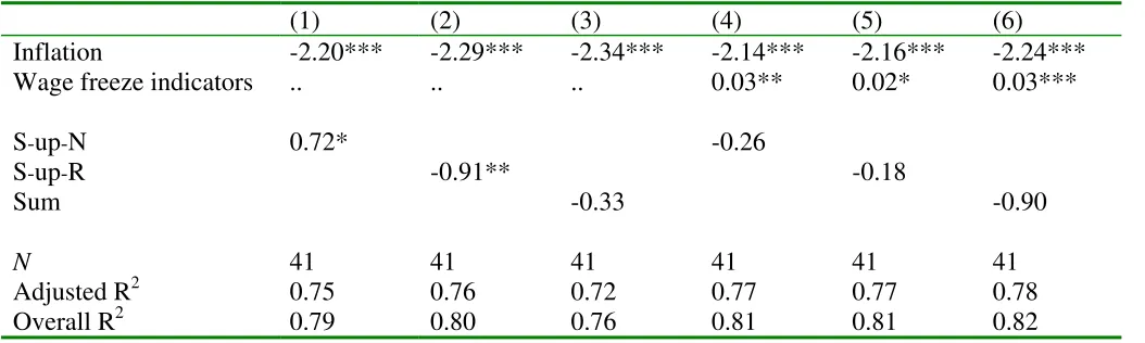
higher unemployment, as predicted by the model of Akerlof et al. (1996). In our baseline
estimations that pool all sectors, sweep up due to nominal rigidity obtains the expected
positive coefficient but sweep up due to real rigidity obtains a negative coefficient (Table 6,
Columns 1-2). However, the time pattern of sweep up measures shows that their behaviour
is related to the changes during the early 1990s. The sweep up measures seem to reflect the
reaction of collective bargaining to the changes in unemployment rather than the effects of
rigidities on unemployment. Nominal wage freeze emerged as a reaction to the increase in
unemployment in the early 1990s. This lead to higher nominal sweep up but to lower real
sweep up as real wage rigidities were relaxed. Consistent with this interpretation, the
amount of real wage sweep up gradually increased during the late 1990s as unemployment
gradually decreased. After adding indicators for the wage freeze years, all statistically
significant results regarding the sweep up measures disappear (Table 6, Columns 4-6). This
confirms that the significance is driven by the depression years (The results using the sweep
up measures that are based on different assumptions about the expected value and the
variance of inflation produce similar findings.)
Taken together, we do not find evidence that the notional mean wage change would be
more sensitive to unemployment than the observed mean wage change. Furthermore, the
extra wage growth due to wage rigidities is not correlated with any extra unemployment.
This indicates that although the measured micro-level real rigidity is high, it is not notably
undermining the adjustment of average wage changes to economic conditions.
VI. Conclusions
This paper studied the micro and macro flexibility of wages in Finland. We covered the
private sector workers by using three data sets from the payroll records of employers’
associations. Two main conclusions emerge. First, there has been macroeconomic
flexibility in the labour market. This means that average wage changes negatively respond
to an increase in unemployment and the downward real rigidity measure declined during
the worst years of the early 1990’s depression. Consistent with this, a large number of
workers experienced a decline in their real wage as unemployment soared. This was put
into effect by wage moderation through collective agreements. However, nominal wage
rigidity increased during the depression and formed the ultimate limit to downward wage
flexibility. Accordingly, we found that lower inflation exacerbates real consequences of
downward nominal wage rigidity. Second, the evidence based on individual-level wage
change distributions reveals that real wages are in general very rigid. Because of the
dominance of collective bargaining, the contract wage rise constitutes a clear cut-off in the
distributions. Hence, it is difficult to separate real wage rigidity from contract wage rigidity.
Alternatively, this indicates that the centralized bargaining institutions are the means that
average wage changes to respond to economic conditions. The evidence also points out that
individual-level wage changes have regained the high levels of real rigidity during the late
1990s that prevailed in the 1980s, despite the continued high (but declining) level of
unemployment.
Regarding the future of wage formation, it is interesting to note that after the depression
union density has declined by more than 10 percentage points in less than ten years. This
rate resembles the decrease in the union density during the Thatcher years in the UK
(Böckerman and Uusitalo 2006). However, this has not led to any increase in real
micro-level wage flexibility, because the union contacts are still almost always extended to
References
Akerlof, G.A., Dickens, W.T. and Perry, G.L. (1996). The Macroeconomics of Low
Inflation. Brookings Papers on Economic Activity, 1, 1-59.
Bewley, T.F. (2007). Fairness, Reciprocity, and Wage Rigidity. In: Diamond, P. and
Vartiainen, H. (Eds.), Behavioral Economics and Its Applications. Princeton: Princeton
University Press, pp. 157-188.
Böckerman, P. and Kiander, J. (2002). Labour Markets in Finland during the Great
Depressions of the Twentieth Century. Scandinavian Economic History Review 50, 55-70.
Böckerman, P., Laaksonen, S. and Vainiomäki, J. (2006). Micro-level Evidence on Wage
Rigidities in Finland. Working Paper No. 219. Labour Institute for Economic Research.
Böckerman, P., Laaksonen, S. and Vainiomäki, J. (2007). Who Bears the Burden of Wage
Cuts? Evidence from Finland during the 1990s. International Journal of Manpower 28,
100-121.
Böckerman, P. and Uusitalo, R. (2006). Erosion of the Ghent System and Union Membership
Dickens, W.T., Goette, L., Groshen, E.L., Holden, S., Messina, J., Schweitzer, M.E.,
Turunen, J. and Ward, M.E. (2007). How Wages Change: Micro Evidence from the
International Wage Flexibility Project. Journal of Economic Perspectives 21, 195-214.
Gorodnichenko, Y., Mendoza, E.G. and Tesar, L.L. (2009). The Finnish Great Depression:
From Russia with Love. NBER Working Paper No. 14874.
Honkapohja, S. and Koskela, E. (1999). The Economic Crisis of the 1990s in Finland.
Economic Policy 17, 400-436.
Koskela, E. and Uusitalo, R. (2006). The Un-intended Convergence: How the Finnish
Unemployment Reached the European Level. In: Werding, M. (Ed.), Structural
Unemployment in Europe: Reasons and Remedies. The MIT Press: Cambridge,
Massachusetts,pp. 159-185.
Kyyrä, T. and Maliranta, M. (2008). The Micro-level Dynamics of Declining Labour Share:
Lessons from the Finnish Great Leap. Industrial and Corporate Change 17, 1147-1172.
Layard, R. and Nickell, S. (1999). Labor Market Institutions and Economic Performance.
In: Ashenfelter, O. and Card, D. (Eds.), Handbook of Labor Economics, Vol. 3C.
Marjanen, R. (2002). Palkkaratkaisujen sisältö ja toteutuminen tulopolitiikan aikakaudella.
(In Finnish). Series B188. The Research Institute of the Finnish Economy.
Nickell, S. and Quintini, G. (2003). Nominal Wage Rigidity and the Rate of Inflation. The
Economic Journal113, 762-781.
Pehkonen, J. (1999). Wage Formation in Finland, 1960-1994. Finnish Economic Papers 12,
82-93.
Sauramo, P. (2004). Is the Labour Share too Low in Finland? In: Piekkola, H. and Snellman,
K. (Eds.), Collective Bargaining and Wage Formation. Performance and Challenges.
Heidelberg: Physica-Verlag, pp. 148-164.
Uusitalo, R. (2005). Do Centralized Bargains Lead to Wage Moderation? Time-series
Evidence from Finland. In: Piekkola, H. and Snellman, K. (Eds.), Collective Bargaining and
Wage Formation. Performance and Challenges. Heidelberg: Physica-Verlag, pp. 121-132.
Uusitalo, R. and Vartiainen, J. (2008). Finland: Firm Factors in Wages and Wage Changes. In:
Lazear, E.P. and Shaw, K.L. (Eds.), The Structure of Wages: An International Comparison.
Chicago: The University of Chicago Press, pp. 149-178.
Vartiainen, J. (1998). The Labour Market in Finland: Institutions and Outcomes.
Table 1. The sensitivity of wage changes to the lagged wage level
Dependent variable: wage change (t)
Manual manufacturing
Non-manual manufacturing
Service sector workers
Wage level (t-2) -0.044*** -0.008*** -0.037***
t-value (-94.02) (-44.59) (-71.46)
N 815 976 877 749 1 162 380
Notes:t-values in parentheses. Significance indicated by *** (1%), ** (5%), * (10%). All
Table 2. The share of workers that have experienced negative wage changes
Nominal wage Real Wage
Manufacturing Manufacturing Services Manufacturing Manufacturing Services
Manual workers
Hourly pay
Non-manual workers
Monthly pay Monthly pay
Manual workers
Hourly pay
Non-manual workers
Monthly pay Monthly pay
1990-1991 16.9 2.0 2.4 60.1 47.8 20.8
1991-1992 36.4 2.7 5.4 69.5 87.2 81.5
1992-1993 20.6 5.4 3.9 57.8 74.4 83.1
1993-1994 8.4 1.4 4.7 11.8 14.5 69.8
1994-1995 5.0 1.2 2.7 6.5 2.3 4.2
1995-1996 10.4 3.3 2.8 12.3 4.8 4.0
1996-1997 23.3 2.7 4.8 48.2 61.3 74.3
1997-1998 11.4 1.3 3.4 18.7 6.4 5.7
1998-1999 11.4 3.5 3.9 17.5 7.6 6.1
1999-2000 6.8 1.6 3.4 33.7 34.9 38.6
Notes: Real wage change is based on actual inflation measured as the annual change in the
Table 3. The amount of nominal and real wage rigidities (averages over several years)
Panel A. Nominal wage rigidities
Manual manufacturing
Non-manual Manufacturing
Services
The late 1980’s 0.00 0.29 ..
The early 1990’s depression
0.44 0.69 0.98
The late 1990’s 0.06 0.31 0.25
Panel B. Real wage rigidities
Manual manufacturing
Non-manual Manufacturing
Services
The late 1980’s 0.29 0.73 ..
The early 1990’s depression
0.04 0.23 0.00
The late 1990’s 0.60 0.70 0.47
Notes: The late 1980’s are 1986-1990, the depression years are 1992-1994 for services and
Table 4. Nickell and Quintini type regressions for the manufacturing manual workers
Dependent variable: the share of negative real wage changes
Median of real wage change -5.42** -4.36**
(-4.26) (-3.86)
Dispersion of real wage changes (P75-P35) -0.96 1.39
(-0.22) (0.38)
Inflation rate 1.49 1.61*
(1.54) (2.01)
Change in inflation rate -1.55 -0.43
(-1.15) (-0.36)
Dummy for the recession years (1991-1993) .. 0.13**
(2.70)
N 19 19
Adjusted R2 0.80 0.86
Table 5. The sensitivity of wage changes to unemployment
Observed mean Estimated mean
Unemployment (t) -0.440** -0.426**
(-5.33) (-4.24)
Productivity growth (t-1) 0.485** 0.503**
(4.11) (3.50)
Expected inflation (t) -0.144 -0.222
(-0.60) (-0.76)
Industry-level bargain 0.018** 0.020**
(3.35) (2.96)
N 41 41
Adjusted R2 0.75 0.67
Notes: Unreported indicators for the sectors and a constant are included. t-values in
Table 6. Sensitivity of unemployment to sweep up due to nominal and real wage rigidity
(1) (2) (3) (4) (5) (6)
Inflation -2.20*** -2.29*** -2.34*** -2.14*** -2.16*** -2.24***
Wage freeze indicators .. .. .. 0.03** 0.02* 0.03***
S-up-N 0.72* -0.26
S-up-R -0.91** -0.18
Sum -0.33 -0.90
N 41 41 41 41 41 41
Adjusted R2 0.75 0.76 0.72 0.77 0.77 0.78
Overall R2 0.79 0.80 0.76 0.81 0.81 0.82
Notes: S-up-N is the magnitude of sweep up due to nominal rigidity computed as -n×(average notional wage change for those with
Figs. 1-6. Wage change distributions
0
.0
5
.1
.1
5
-20 -15 -10 -5 0 5 10 15 20
Blue Collar
Wage Change Centered on Contract Wage
0
.0
5
.1
.1
5
-20 -15 -10 -5 0 5 10 15 20
Blue Collar
0
.0
5
.1
.1
5
.2
.2
5
.3
-20 -15 -10 -5 0 5 10 15 20
White Collar
Wage Change Centered on Contract Wage
0
.0
5
.1
.1
5
.2
.2
5
.3
-20 -15 -10 -5 0 5 10 15 20
White Collar
0
.0
5
.1
.1
5
.2
.2
5
.3
-20 -15 -10 -5 0 5 10 15 20
Services
Wage Change Centered on Contract Wage
0
.0
5
.1
.1
5
.2
.2
5
.3
-20 -15 -10 -5 0 5 10 15 20
Services
Fig. 7. Actual inflation and the median wage change by sector
0 0.01 0.02 0.03 0.04 0.05 0.06 0.07 0.08 0.09 0.1
1986 1987 1988 1989 1990 1991 1992 1993 1994 1995 1996 1997 1998 1999 2000 2001
Appendix A: Data description
We use ‘wage surveys’ of two Finnish employers’ associations. Manufacturing sector
manual (hourly paid) blue-collar workers and non-manual (salaried, monthly paid)
white-collar workers are covered by TT (Teollisuus ja työnantajat). The private service sector
workers are covered by a survey of PT (Palvelutyönantajat). Wage information in these
surveys originates directly from the payroll records of companies. Thus, they can be
characterised as administrative or register based data. These data are very accurate, and
the measurement error in surveys of individual workers, like recall or rounding error, is
not a significant problem.
The survey frame of the data consists of the member firms of both associations in each
reference period. Although the survey is mandatory for firms with over 30 workers (the
limit varies somewhat by industry), some non-response will occur. This is concentrated
on smaller firms that are also less often members of the associations. The coverage of
the TT data is better than that of PT, since service firms are smaller on average. To
identify employers in TT data there are firm codes and ‘response-unit’ codes. There has
been a break in the firm coding system during our observation period, but the response
unit codes are consistent over time. Thus, we use those to identify the employer of
individuals. The response-unit refers to the establishment of a firm. In the service sector
only the firm code exists in the data, so we use it.
The data are well representative at the worker level, since the TT/PT firms have good
electronic systems for collecting wage data. There are some missing or erroneous
identity codes. Those individuals are excluded from wage changes. However, after the
The structure of these data is quite similar across sectors. They provide information
about wages and working time, and some information about workers’ individual
characteristics (such as age and gender). However, there are two major differences in
these data sets across the sectors: the timing of observations and the wage concept. For
manual manufacturing workers the data covers the situation during the last quarter of each
year for the period 1981-2000, but the situation during one month of each year for
non-manual (salaried) manufacturing workers (September before 1993 and December in and
after 1993) for the period 1985-2000 and the private service sector workers (August
before 1995 and October in and after 1995) for the period 1990-2001. This change-over
causes no major problems because the observation month is delayed and there is a point of
normal contractual wage increase between the two observations (otherwise we might
overestimate downward rigidity). We might underestimate the rigidity by lengthening the
observation interval if more than the usual one or two annual contract wage rises fell on the
interval. However, this is not the case for either sector. The observation interval changes
only by two or three months, so the change-over years should be comparable to other
years.
The wage concept differs across sectors. Hourly rate has been applied for manual
workers in manufacturing, whereas monthly rate (salary) for non-manual workers in
manufacturing and for service sector workers. The monthly rate for non-manual workers
in manufacturing is defined as ‘the fixed basic monthly salary paid for regular working
time’. This fixed salary is based on the ‘demands’ of the job or tasks performed in it and
the contract-based wages determined for these ‘demand classes’ of jobs, and an
additional person-specific component based on personal competence. Respectively, in
time’, which is very close to the former definition. It includes such personal and ‘task’
specific bonuses (merit pay), which are paid at the same amount in each month. These
monthly wages exclude such components of wages, which are inherently chancing or
are not part of the ‘basic wage’ of a person. Excluded are among others overtime pay,
shift work, evening or Sunday bonuses, fringe benefits, and performance based
payments, commissions, ‘profit sharing’ and similar payments. It should be noted, that
the monthly wage is not simply a ‘minimum’ salary based on contracted wage scales,
but includes a person-specific component. Firms and local unions can also agree on
firm-specific wages that exceed the minimum requirements of national contracts. Such
firm-specific arrangements can be reduced by mutual consent of the firm and local
union. These person and firm-specific components in wages provide possibilities for
both upward and downward flexibility in wages.
For measuring hourly rate for manufacturing manual workers there are two options: the
wage per hour for regular working time, or the wage per hour for straight time work
(time-rate). We use the time-rate, because it is a better measure of the person’s ‘basic’
wage. The regular-time measure includes compensation from all types pay, that is,
time-rate, piece-rate and performance based pay. Therefore, it can change if the structure of
hours of work performed as time work, piece-rate work or performance work change.
Such wage changes reflect changes in person’s work effort which is problematic for the
purposes of studying downward rigidity of wages. A wage cut arising from less hours or
less effort in piece-rate work is not what is meant by flexible wages, which refers to
changes in the ‘basic wage’ of persons. Therefore, we use thehourly wage measure for
time-rate work. It is calculated by dividing the wage bill for time-rate hours by hours
quarter of each year. This hourly wage measure excludes piece-rate and performance
work, overtime pay (and hours), and shift work, evening, night and Sunday bonuses, as
well as bonuses based on working conditions. It includes any firm-specific wages paid
above minimum contracts, and any ‘personal bonus’ incorporated in each person’s
individual ‘wage rate per hour’ that is used in remuneration for his/her time-work.
Again, these person and firm-specific components in wages provide possibilities for
both upward and downward wage changes, and deviations from the wage changes in
centrally negotiated contracts.
A drawback of using the time-rate hourly wage is that it leads to the omission of small
number individuals from the data, who are 100% paid on piece-rate or performance pay.
The straight time hourly wage can also be based on few hours, but it is not clear that this
should produce any problems as such, as long as the wage bill and hours data are
otherwise accurate.
The wage changes are constructed for job stayers, that is, only workers who have the
same employer and the same occupation during the two consecutive years are included.
It is standard in micro-level studies of wage rigidity to restrict to the wage changes of
persons who remain in the same job (e.g. Bewley 2007). Wage changes related to job
promotions or demotions and employer switches reflect changes in job tasks, working
conditions and location amenities, which contaminate measurement of wage rigidity. To
control for the variation arising from changing working hours for non-manual and
service sector workers’ monthly wages, it is required that the “regular weekly hours” are
1
This paper is based on the analyses of the project Wage Rigidity and Labour Market Effects of Inflation financed by the Finnish Work Environment Fund. Part of the results draw upon work conducted in the International Wage Flexibility Project. We are grateful for the IWFP leaders and partners for co-operation and comments. All errors remain our responsibility.
2
The centralized framework was abandoned only during 2008-2009 wage negotiations. Employers’ associations repealed their central organization the right to agree upon wage contracts with corresponding workers’ organization.
3
Appendix A provides a description of the data sources. Uusitalo and Vartiainen (2008) examine the changes in wage structure in Finland by using the same data.
4
Böckerman et al. (2006) document the annual distributions.
5
There was an attempt by the social partners to cut nominal labour costs by 7% in 1991 in order to avoid currency depreciation. (The proposition to cut labour costs by 7% included 3% cut in nominal wages and 4% transfer of pension contributions from employers to workers.) However, this attempt failed because two major unions delayed their support for the pact and the financial markets forced the Bank of Finland to abandon the fixed exchange rate in November 1991. After that episode the labour market organizations did not accept any cuts in nominal wages, but agreed, for the first time since the Second World War, to a two-year social pact without any nominal pay rises.
6
7
Details for the justification of using Weibull distribution can be found in Dickens et al. (2007). Briefly, examination of the wage change distributions in the IWFP project (and some other researchers) indicates that wage change distributions are more peaked and have fatter tails than the normal distribution. Second, the upper half of the distribution (above median), which is presumably not affected by wage rigidities, is well approximated by a Weibull distribution.
8
To quantify the amount of rigidities it is necessary to make additional assumptions about the way that wage rigidities transform the notional wage change distribution to the observed distribution. Without rigidities we would observe the notional wage change distribution which is assumed to be symmetric. A fraction of the population is subject to downward real wage rigidity, if their notional wage change is below the expected rate of inflation, and they receive a wage change equal to that expected rate of inflation rather than equal to their notional wage change. The mean and standard deviation of the expected rate of inflation in each year are parameters of the protocol and they are estimated separately for each year. We use estimates in which the expected value and the variance of expected inflation are both constrained (standard deviation constrained to be less than 0.6%). A fraction of the population is also potentially subject to downward nominal wage rigidity. Such workers who have a notional wage change less than zero, and who are not subject to downward real wage rigidity, but who receive a wage freeze instead of a nominal wage cut, are affected by downward nominal rigidity. See Dickens et al. (2007) for details.
9
We use the data for manual manufacturing workers, because the data are available for a longer period (1981-2000) only in this sector, which is necessary to have enough variation in inflation.
10