AN EFFICIENT EVOLUTIONARY ALGORITHM FOR LOCATING LONG-TERM CARE FACILITIES

(1)

An efﬁcient evolutionary algorithm for locating long-term care facilities

Zorica Stanimirovi´c

Faculty of Mathematics, University of Belgrade, Studentski trg 16/IV, 11 000 Belgrade, Serbia

e-mail: [email protected]

Miroslav Mari´c

Srdjan Božovi´c

MFC-Mikrokomerc, Zaplanjska 86, 11000 Belgrade, Serbia

Predrag Stanojevi´c

Abstract. This paper deals with a variant of a discrete location problem of establishing long-term care facilities in a given network. The objective is to determine optimal locations for these facilities in order to minimize the maximum number of assigned patients to a single facility. We propose an efficient evolutionary approach (EA) for solving this problem, based on binary encoding, appropriate objective function and standard genetic operators. Unfeasible individuals in the population are corrected to be feasible, while applied EA strategies keep the feasibility of individuals and preserve the diversity of genetic material. The algorithm is benchmarked on a real-life test instance with 33 nodes and the obtained results are compared with the existing ones from the literature. The EA is additionally tested on new problem instances derived from the standard ORLIB AP hub data set with up to 400 potential locations. For the first time in the literature we report verified optimal solutions for most of the tested problem instances with up to 80 nodes obtained by the standard optimization tool CPLEX. Exhaustive computational experiments show that the EA approach quickly returns all optimal solutions for smaller problem instances, while large-scale instances are solved in a relatively short CPU time. The results obtained on the test problems of practical sizes clearly indicate the potential of the proposed evolutionary-based method for solving this problem and similar discrete location problems.

Keywords:Evolutionary algorithms; Long-term care facility; Facility location problem; Discrete optimization.

1. Introduction

There are many research articles on facility lo-cation problems which arise from designing and op-timizing health-care systems and health-care service delivery. The use of Operational Research (OR) in health-care has developed signiﬁcantly in the past decade; namely, both the number of OR applications in this area and the number of topics covered have increased. Recently, the OR applications have moved

systems are country-specific, which is an important influential factor in the health care industry. Countries which have market-oriented health care systems tend to put more effort into service improvement, in or-der to increase the number of customers. On the other side, countries with a budget-oriented system put pri-ority on improving efficiency and decrease the wait-ing lists of patients.

In the literature there are numerous OR problems http://dx.doi.org/10.5755/j01.itc.41.1.1115

(2)

in real OR problems which include the sitting and re-sponse of emergency services, such as medical ser-vice, police, fire stations, see [9], [13] and [27]. In the paper by Brotcone et al. [5], one can find a re-view of FLM application in emergency response ser-vices. Facility location models may be divided in cov-erage and median type models [3]. Median models locate the emergency-services and allocate customers to them in order to minimize average or total travel time/cost in the emergency-service network. Cover-age models deal with the location of services so that adequate coverage is provided to customers, imply-ing that there is at least one service that can satisfy a demand of a user in a position within a preset max-imum distance. Covering models are mostly used to describe location problems in emergency-service ap-plications. Numerous covering models with various problem-specific constraints are proposed for both mobile and fixed emergency services. The most com-mon objectives in these problems are to minimize the maximal waiting time of a customer, minimize the number of facilities or emergency vehicles, determine the locations of emergency service facilities required to satisfy the demand for the service. A review of these problems can be found in [8], [22] and [26].

In this paper, we focus our research to an OR problem which, in the objective function, involves a workload balance of the health-care facilities. There are several location problems in the literature dealing with this or similar OR problems. In papers by Boffey et al. [4] and Galvao et al. [10], the authors consider a problem of location of perinatal facilities in the mu-nicipality of Rio de Janeiro. Their research lead to the development of an uncapacitated, three-level hi-erarchical model, denoted as the "basic model". The overall objective was to contribute to the reduction of perinatal mortality in the municipality through a bet-ter spatial distribution of health care facilities. Bof-fey et al. in [4] make clear that this model is an ide-alisation of real-life situation, which neglects details such as capacity constraints, aggregation of adjacent neighborhoods, political boundaries and social fac-tors, which might be of signiﬁcance in practice. The incorporation of some form of capacity constraints into the model is shown by the authors to be a crit-ical point.

Galvao et al. in [11] and [12] further discuss practical aspects in location problems of balancing loads of maternal health-care facilities considering both the uncapacitated and capacitated cases. Au-thors extend "basic model" to hierarchical models with a bi-criterion objective for the location of ma-ternal and perinatal health care facilities in Rio de Janeiro. A 3-level uncapacitated hierarchical model

was initially developed and capacity constraints were later added to the resource intensive level of the hier-archy. A bi-criterion model of minimizing total travel distance and load imbalance in a 3-level hierarchical system was developed in an attempt to balance the load among level 3 services. The authors proposed Lagrangean heuristics for solving both the uncapac-itated and capacuncapac-itated models. The results obtained with the uncapacitated model produced a good spa-tial distribution of the perinatal health care facilities at the three levels of the hierarchy. The capacitated model was used in a case study that allowed capacity planning issues to be analysed.

In this paper, we consider one particular discrete optimization problem, named the Long-Term Care Facility Location Problem (LTCFLP). We start with a given setJof potential facility locations, assuming that no facility is previously established. The set of potential facility sites coincides with the set of patient groups, which means that a facility may be located at one of the locations of the patient groups. The ele-ments of the setJwill be referred to as "nodes". The objective is to locate a certain number of long-term facility sites, in order to minimize the maximum load of established facilities. We assume that all potential facilities have the same capacity, that is, the numbers of sickbeds in the facilities are the same. We spec-ify the locations and demand quantities (the number of patients) for each patient group. The problem in-volves a single allocation scheme, which means that each patient group is assigned to exactly one, previ-ously established facility. All patients in each patient group are to be served by a facility located nearest to the location of the patient group. The maximum num-berKof facilities to be established is pre-determined, and the inequalityK≤ |J|holds. No capacity restric-tions on the established facilities are assumed. Fixed costs for locating facility sites are not considered in this model.

(3)

by adopting and modifying the add, drop and inter-change methods and by applying them sequentially. The solution generated by the MADI heuristic is used as an upper bound in the branch and bound method (BnB). For evaluation of the suggested algorithms, computational experiments are performed on a real problem with|J|=33 locations in a province in Ko-rea and a number of problem instances with up to

|J|=70 locations and different levels ofK. The so-lutions of the proposed algorithms are additionally compared with the solutions obtained by the opti-mization software package CPLEX [7], version 10.0. CPLEX Optimizer is a high-performance mathemat-ical programming solver developed for solving lin-ear programming, mixed integer programming, and quadratic programming problems to optimality. Re-sults of the experiments show that the suggested BnB algorithm gives optimal solutions on problem in-stances with up to|J|=40 nodes, while the MADI heuristics produces solutions with certain gaps from the optimal ones. Among 15 problems with 50−70 patient groups, 10 problems were solved to optimal-ity by the BnB algorithm. In other cases, neither BnB nor CPLEX 10.0 reached optimal solutions after 24 hours of computational run. For most of the instances with 50−70 nodes, the MADI heuristic produced so-lutions with signiﬁcant gaps from the optimal or best known solutions.

In the literature, one can ﬁnd similar location problems that involve minimization of the maximal load of a facility under certain conditions. Baron et al. [1] consider the problem of locatingM facilities per square unit so as to minimize the maximal load of the facilities, subject to closest assignments and coverage constraints. Focusing on a uniform demand per square unit, the authors develop upper and lower bounds on feasibility of the problem and suggest a heuristic to solve the problem. Marin in [23] deals with a discrete facility location problem where the difference between the maximum and minimum num-ber of customers allocated to every plant has to be balanced. Two different integer programming formu-lations are built, and several families of valid inequal-ities are developed and incorporated in a branch-and-cut algorithm. The research presented in this study was motivated by the potential of evolutionary strate-gies that were previously applied to various facility location problems: hub location problems [6], [17], [20], [21], [30], [31], [32], hierarchical covering loca-tion problems [24], discrete ordered median problem [29], multi-level facility location problem [25] etc. Although some of these problems have similar for-mulations, their properties are substantially different and the proposed evolutionary algorithms for solving

them have quite different nature. In some cases, the evolutionary approach designed for one facility loca-tion problem may be theoretically applied to another problem, but the results are often far from optimal ones, even for small size instances.

In this paper, we propose an evolutionary-based algorithm (EA) for solving the LTCFLP. We use bi-nary representation of solutions and appropriate evo-lutionary operators. The EA is enriched with several strategies that correct and keep the individuals fea-sible, preserve the diversity of individuals and pvent premature convergence of the algorithm. The re-mainder of the paper is organized as follows. In Sec-tion 2, we present a mathematical formulaSec-tion of the LTCFLP. Section 3 explains in detail all important as-pects of the proposed evolutionary algorithm. In Sec-tion 4, we present and discuss the results of the EA implementation on a real-life problem instance with 33 nodes, presented in [19]. The algorithm is also benchmarked on the newly generated data set, based on the AP hub instances from the ORLIB library [2]. The new LTCFLP instances have up to 400 potential facility locations and involve different levels ofK. We compare the performance of the proposed EA with the exact BnB method and the MADI heuristic from [19] on the available common set of test instances. Fi-nally, in Section 5, we draw out some conclusions and propose ideas for future work.

2. Mathematical formulation

In this paper, we start from the mixed-integer for-mulation of the LTCFLP given in [19]. LetJbe a set of candidate facility locations.di jrepresents the

dis-tance between the location of a patient groupiand a candidate facility location j, whileaiis the number of

patients in a patient groupi. An integer numberK>0 denotes the maximum number of facilities to be lo-cated, andM>0 is a large constant. We introduce a decision binary variableyj∈ {0,1}that is equal to 1

if a facility is established at the candidate facility lo-cation j, and 0 otherwise. A decision binary variable xi j∈ {0,1} takes the value of 1 if a patient groupi

is allocated to a facility location j and 0 otherwise. Non-negative variableLmax represents the maximum

load of the established long-term care facility sites. Using the notation mentioned above, the problem can be formulated as:

min Lmax (1)

subject to:

∑

j∈J

xi j=1 f or every i∈J (2)

(4)

xi j≤yj f or every i,j∈J (3)

∑

l∈J

dilxil≤di j+M(1−yj) f or every i,j∈J (4)

∑

j∈J

yj≤K (5)

∑

i∈J

aixi j≤Lmax f or every j∈J (6)

xi j∈ {0,1} f or every i,j∈J (7)

yj∈ {0,1} f or every j∈J (8)

The objective function (1) minimizes the max-imum load of established facilities for load balanc-ing. The constraint (2) guarantees that each patient group is allocated to exactly one facility location. The constraint (3) restricts such assignments to be made only to previously established facilities. Each patient group is assigned to its nearest facility, which is en-sured by the constraint (4). Constraint (5) guarantees that the total number of established facilities does not exceed a predetermined integer constantK>0. Con-straint (6) deﬁnes the lower bound for the objective variableLmax, which represents the maximum load of

established facilities for load balancing. Finally, (7) and (8) indicate binary nature of variablesxi jandyj

respectively.

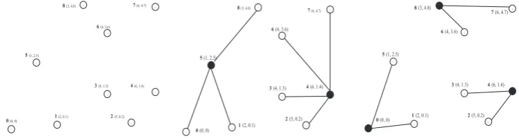
Example 1: On the left side of Figure 1, we present one example of a network with n=9 nodes, denoted as (0,1,...,8). Each node is given by its (x,y) coordinates in the plane, representing one pa-tient group. The number of papa-tients in a group that is assigned to each node is given by the vector (100,60,210,90,70,230,150,20,190).

Solving the LTCFLP with up toK=2 andK=3 located facilities, we obtain optimal solutions, which are presented on the right side of Figure 1. In case of K=2, facilities are located at nodes 4 and 5. Each pa-tient group is allocated to its nearest facility: groups 2, 3, 4, 6, 7 are associated with facility 4, while groups 0, 1, 5, 8, are allocated to facility 5. The loads of es-tablished facilities at nodes 4 and 5 are 540 and 580 respectively. The objective value (maximum) is ob-tained for facility 5 (580 patients)

If we slightly increase the maximal number of facilities to be located to K=3, the objective func-tion decreases to the value of 390. Facilities are es-tablished at nodes 0, 4 and 8. Patient groups at nodes 0, 1 and 5 are assigned to facility 0, groups 2, 3, 4

to facility 4 and groups 6,7,8 to facility 8. Since the loads of facilities 0, 4 and 8 are 390, 370 and 360 re-spectively, it can be seen that the objective function value is achieved for the facility 0 (390 patients).

3. Proposed evolutionary algorithm

3.1. Representation and objective function

In this EA implementation, a binary encoding of individuals is used. Each solution is represented by a binary string of lengthn, wheren=|J|. Each bit in the genetic code corresponds to one node in the network. If the j-th bit in the genetic code takes the value of 1, it denotes that a facility is located at the j-th node, while 0 indicates it is not. Note that the enumeration starts from zero, i.e. j∈ {0,1,...,n−1}.

From the genetic code we obtain the locations of established facilities, i.e. the indices j whereyj=1,

j∈ {0,1,...,n−1}. Once the locations of facilities are determined, patient groups can be easily assigned to the facilities. The values of xi j,i= j can be

de-termined directly by comparing the distancesdi j

be-tween the established facilities and location of each patient group. Finally, the objective value (1) is sim-ply evaluated by comparing the loads of the estab-lished facilities and determining the maximal one.

Example 2: The genetic code(0|0|0|0|1|1|0|0|0|) corresponds to the optimal solution forn=9,K=2 presented in Figure 1. From the genetic code we obtain indices of located facilities 4 and 5, which gives us the variablesyj:y4=y5=1 andyj=0,j∈

{0,1,...,8},j=4,5. Patient group at each established facility is obviously assigned to itself (i.e.xii=1⇔

yi =1), while the values of variables xi j,i= j are

obtained by comparing the distances from a patient groupito established facilities 4 and 5. The optimal solution forn=9,K=3 in the Example 1 is repre-sented by the binary string (1|0|0|0|1|0|0|0|1|). The positions of 1 in the genetic code indicate that facil-ities are sited at nodes 0,4 and 8. It means thaty0=

y4=y8=1 andyj=0,j∈ {0,1,...,8}, j=0,4,8. It

follows thatx00=x44=x88=1, whilexi j,i= jare

obtained in the same way as described before.

3.2. Construction of initial population

Initial EA population, numberingNpop=150

in-dividuals, is randomly generated. This approach pro-vides maximum diversity of genetic material and a better gradient of the objective function. Initial solu-tions are created randomly by setting each bit in the genetic code with certain probability.

(5)

7 (6, 4.7) _{8 (3, 4.8)}

c

0 (0, 0) 1(2, 0.1) 2(5, 0.2) 3(4, 1.3) 4(6, 1.4) 5(1, 2.5)

6(4, 3.6) 8 (3, 4.8)

c

c c

c

c c

c

0 (0, 0) 1 (2, 0.1)

2(5, 0.2)

3(4, 1.3) 4(6, 1.4)

5(1, 2.5)

6(4, 3.6)

c

c c

c

c c

c

c 7 (6, 4.7)

c

0 (0, 0) 1(2, 0.1) 2(5, 0.2)

3(4, 1.3) 4(6, 1.4)

5(1, 2.5)

6(4, 3.6)

7 (6, 4.7)

c

c c

c

c c

c

c 8 (3, 4.8)

Figure 1. Optimal solutions on a network withn=9 nodes andK=2 andK=3 facilities

larger. In order to provide better quality of initial pop-ulation and direct the algorithm to better search re-gions, we deﬁned the probabilitypof generating ones in the individual’s genetic code as a function of the problem parametersnandK, i.e.p=K_n.

It may happen that incorrect individuals, which have M >K ones in their genetic code appear in the population. These individuals may be generated in the initial population, or created by applying the crossover or mutation operators. Incorrect individuals may become dominant in the population and signiﬁ-cantly increase the possibility of premature conver-gence. Instead of discarding the incorrect individu-als from the population, we correct them by changing M−K ones to zeros from the end of genetic code. In this way, we keep the feasibility of the individuals through an EA generation and prevent the EA from loosing some regions of the search space.

3.3. Evolutionary operators

In the proposed EA method, we used the fine grained tournament selection introduced in [16]. A classic tournament selection operator ([18], [33]) is realized through tournaments of constant sizetour. The basic idea of the fine grained tournament selec-tion is to involve tournaments with different number of competitors in the same EA generation. In this EA implementation, the selection operator is realized by using two types of tournaments. The first tourna-ment type is heldk1times and its size isavgtour.

The second type is performed k2 times with the

avgtour individuals participating. The rational pa-rameter avgtour represents the average tournament size, i.e. avgtour=k1avgtour+k2avgtour

k1+k2 . In our

im-plementation,avgtouris set to 6.4, which means that we realize k1=20 tournaments of size 6.4=7

andk2=30 tournaments of size6.4 =6. The

run-ning time for the implemented selection operator is O(nind·avgtour), wherenind=number of selected

in-dividuals. In practice, avgtour is considered to be constant (not depending on number ofnind), that gives

O(nind) time complexity.

After a pair of parents is selected, the crossover operator is applied to them producing two offspring. Standard one-point crossover exchanges segments of two parents’ genetic codes after the crossover point that is randomly chosen. The crossover is performed with the rate probability crossrate= 0.85. It means that around 85% pairs of individuals take part in pro-ducing offspring.

In the later EA stages, it may happen that all in-dividuals in the population have the same bit value on some position in the genetic code. On the Figure 2 we present an example of the EA population of 7 individ-uals with genetic codes of lengthn=10, which gives us a search space of the size 210. As it can be seen from the Figure 2, the bit values on positions 1,7 and 9 are the same (frozen bits), which produces the re-duction of the initial search space by the factor of 23. The appearance of frozen bits significantly increases the possibility of premature convergence. By apply-ing the crossover operator, no frozen bit value can be changed, while a simple mutation operator is not efficient enough to restore the lost regions of search space, due to the low mutation rates. If we increase the mutation rate significantly, the EA may loose its essence and turn into random search.

For this reason, we apply a modified mutation operator with frozen bits, i.e. we increase the muta-tion rate on frozen bits only, by multiplying it with a certain "frozen" factor. In each EA generation the mutation operator goes through genetic codes of in-dividuals and identifies the positions of the potential frozen bits. On non-frozen bits, we apply a lower (ba-sic) mutation rate of 0.4/n, while the mutation rate for frozen bits is multiplied by the "frozen" factor=4.0 and is equal to 1.6/n. Neither mutation rate changes through an EA run. This approach showed to be more efficient for this problem compared to the standard simple mutation operator, as in [15] and [33].

3.4. Population replacement and stopping criteria

(6)

individual 1: 0100011100

---bit position: 0123456789

Figure 2. Frozen bits, n=10, K=5

through the search space and to improve its efﬁciency. Applied strategies help in preserving the diversity of the genetic material and in keeping the algorithm away from a local optima trap.

In the proposed EA method, we use steady-state generation replacement scheme with elitist strategy, which consists of copying some of the best individ-uals in the current population to the new population. In every EA generation, all individuals are ranked ac-cording to their objective function value. The best-ﬁtted 100 individuals are denoted as "elite" ones and they directly pass into the next generation, thus pre-serving highly ﬁtted genes. The remaining 50 individ-uals, named "non-elite" ones, are subject to EA opera-tors and they are replaced in the next generation. Note that elite individuals do not need recalculation of the objective value since each of them is evaluated in one of the previous generations. An individual with the best objective value is denoted as the "best individual" and its value and the corresponding genetic code are saved separately. The "best individual" is being up-dated through EA generations, whenever we achieve some improvement of the best objective value.

The advantage of the elitist strategy over the tra-ditional approach, where an entire population is com-pletely replaced with new chromosomes, is that the best individual in the population is monotonically im-proving over time. A potential disadvantage is an in-creased similarity of individuals in later EA genera-tions, which may cause convergence to a local mimum. However, this problem was overcome by in-creasing mutation rates on frozen bits (Section 3.3.)

Duplicate individuals are discarded from the population. The objective value of a duplicate individ-ual is set to zero and the selection operator disables it to enter the next generation. The individuals with the same objective value, but different genetic codes may dominate in the population after a certain number of iterations. If their codes are similar, it may cause a premature convergence of the EA. For that reason, we keep only 40 individuals with the same objective value, but different genetic codes in the population.

A combination of two stopping criteria are used for EA: maximum number of generations -Gmax =

1500000 and maximum number of best code’s repeti-tion -Rmax=500000. In order to enhance and assess

the reliability of the EA performance, each test in-stance is replicatedN=20 times. The basic scheme of the Evolutionary method is as follows:

EA method {

Initialization:

Define the representation of solutions; Choose the stopping criteria: G_max, R_max; Generate an initial population P;

iter=1; rep=1;

while ((iter ≤ G_max) && (rep ≤ R_max))

{

For each solution X ∈ P do Ob jective_Function(X); Selection;

Crossover; Mutation;

if ((iter≥ 1)&&(BestSol(iter−1) ==BestSol(iter)))

then rep=rep+1; iter=iter+1;

} }

4. Computational results

In this section, the computational results of EA and comparisons with existing algorithms are pre-sented. All experiments were carried out on an Intel Core i7-860 2.8 GHz with 8GB RAM memory under Windows 7 Professional operating system. The EA implementation is coded in C programming language. Computational experiments were ﬁrst performed on a problem instance with 33 nodes, which was de-rived from a real situation in Korea and introduced in [19]. Each district of Korea is represented by a node (candidate facility location or a patient group), which is given by its (x,y) coordinates in the plane. Dis-tances between pairs of nodes are calculated as the Euclidean distances between them. Forecasted num-ber of patients is assigned to each potential facil-ity location. The maximum number of facilities to be established K is varied, since it can be affected and changed by the budget and health-care policy of the government. In our experiments, the parame-terKtakes seven values(4,8,12,16,20,24,28), as in [19]. Because of the small problem dimension, we de-creased the parameter values for stopping criterion to Gmax=1600 andRmax=500. The EA was runN=20

(7)

The results of our EA implementation, the BnB method and heuristic approach from [19], together with the corresponding total CPU times are presented in Table 1. Note that the BnB method and heuristic method were tested on a Pentium processor operat-ing at 3.2 GHz. The optimal solutions on this data set were obtained by CPLEX 10.0 solver (which was run on the same processor) and taken from [19].

Column headings of Table 1 mean:

• Instance’s parameters: number of nodes n=|J|andK;

• Optimal solution of the current instance -Opt.Solobtained by CPLEX 10.0 solver;

• Total CPLEX 10.0 running time in seconds -CPUt;

• The best value of EA method on the current instance -EAbest, with markoptin cases

when it reached optimal solution;

• Running time in which the EA reachesEAbest

for the ﬁrst time -CPUstartin seconds;

• Total running time of the EA -CPUendin

seconds;

• Average percentage gap -agapofEAbest

solution from theOpt.Sol;

• Average number of EA generations -Ngen;

• The total running time of the BnB method -BnBtin seconds;

• The best solution of the heuristic method Heurbest;

• The percentage gap of the solution of the heuristic from the optimal oneHeurgap;

• The total running time of the heuristic Heur -Heurtin seconds.

As it can be seen from Table 1, the proposed EA quickly reaches all optimal solutions in average 0.246s of total CPU time. Average time in which the EA detects the optimal solution for the ﬁrst time is around 7 times shorter-0.0346s. The EA has obvi-ously better performance compared to the Modiﬁed Add-Drop-Interchange heuristic algorithm (Heur), in the sense of solution quality. The proposed heuristic doesn’t achieve optimal solutions forK=4,8,16 and produces an average gap of 0.829%.

The average gap is calculated asagap=_N1

N

∑

i=1

gapi,

whereN represents the number of EA runs on the same instance (N =20), while gapi represents the

gap of an EA’s solution soli obtained in the i−th

run, i=1,2,...N. Note that gapi is evaluated with

respect to the optimal solutionOpt.Sol, i.e. gapi=

100soli−Opt.Sol

Opt.sol , or the best-known solutionBest.Sol,

i.e.gapi=100soli_Best−Best_._Sol.Sol in cases when no optimal

solution is known. In the cases of tested instances in

Tables 2-7 for which optimality was not proven, the best known solution is actually the best EA solution: Best.Sol=EAbest.

In order to provide fair comparisons of CPU times, we run a set of preliminary experiments of the EA on a subset of the newly generated instances using a processor Pentium(R)IV 1.8GHz with 504 MB RAM under Windows XP professional operat-ing system. Accordoperat-ing to SPEC fp2006 and fp2000 benchmarks (www.spec.org), this configuration has around two times slower performance compared to the one used in [19]. Detailed computational results, presented on the web site http://www.matf.bg.ac.rs/∼ maricm/ltcflp/PerformanceComp.pdf, show that the Intel Core i7-860 2.8 GHz with 8GB RAM has ap-proximately 3 times better performance (on average) compared to the Pentium IV 1.8GHz with 500 Mb. Based on these facts, we may conclude that the con-figuration used in this paper performs around 1.5 times better than the one from [19].

If we multiply the average EA’s total CPU times by the factor of 1.5, we obtain 0.246∗1.5=0.369s, which is around 21 and 234 times shorter time com-pared to the average running times of CPLEX 10.0 and BnB method respectively. It turns out that the heuristic Heur is around 1.8 times faster than the EA, but the solution quality of it is lower compared to the EA.

In the paper [19], the authors also performed experiments on the problem instances that were generated randomly by varying the values of |J| and K. They generated test problems with |J| = 20,30,40,50,60,70 nodes and included ﬁve levels of K for each problem size |J|. Unfortunately, these problem instances remained unavailable to us.

4.1. Results on modiﬁed AP data set with50≤n≤

200nodes

In order to evaluate the performance of the pro-posed EA on a wider range of problems, we used the standard ORLIB AP data set to perform additional se-ries of tests. The AP (Australian Post) data set was introduced by Ernst and Krishnamoorthy in [14] and is considered to be a benchmark by most researchers in the hub location area. It is derived from the real-world application of a postal delivery network and consists of 200 nodes given by their (x,y) coordi-nates, the ﬂow matrix with demands for each pair of nodes, capacity restrictions and ﬁxed costs for each node. Smaller size AP instances are obtained from this instance by aggregating the initial set ofn=200 nodes.

(8)

Table 1. Results and comparisons of the EA on small-size instances|J|=33

K Opt.Sol CPUt EAbest CPUstart CPUend agap Ngen BnBt Heurbest Heurgap Heurt

4 3610 19.85 opt 0.083 0.216 0.065 859.5 1.14 3646 1.0 0.05 8 1993 15.14 opt 0.026 0.217 0.04 833.6 101.69 2001 0.4 0.09 12 1440 7.55 opt 0.03 0.227 2.264 858.4 171.92 1440 0.0 0.17 16 1079 4.92 opt 0.103 0.289 0.222 1105.5 68.45 1127 4.4 0.27 20 1079 3.68 opt 0.0 0.212 0.0 753 179.14 1079 0.0 0.25

24 1079 3.03 opt 0.0 0.22 0.0 751 76.69 1079 0.0 0.30

28 1079 2.04 opt 0.0 0.339 0.0 751 6.45 1079 0.0 0.25

avg 8.030 0.0346 0.246 0.370 844.6 86.497 0.829 0.197

sents potential long-term health facility location or a patient group. For AP instances withn=50,100,200 nodes we used the given capacities (tight-T and loose-L) as the demands of the nodes for the LTCFLP (the number of patients in each patient group). Since for AP instances withn=60,70,80,90,110,120 and 130 nodes no capacities are given, for each instance we add two types of patient demandsa(i)on each node, based on the incoming, outcoming node’s ﬂow and to-tal ﬂow in the network. More precisely, demands are obtained by the following formula:

a(i) =W∗(D(i)/(O(i) +D(i)))∗(1±r),

whereW = total ﬂow in the network,O(i),D(i) = outcoming and incoming ﬂow for nodei, whiler= randomly chosen number from the interval(0,0.5). Loose and tight demand types are denoted as L and T respectively. The values ofK were set to integers 20≤k≤ |J| −10.

The report of all computational experiments that are performed is too large for this paper. Therefore, in Tables 2-5 we present our results on a chosen subset of tested instances, while the complete report may be found on the web site

http://www.matf.bg.ac.rs/∼maricm/ltcﬂp/

DetailedCompReport.pdf. The results are presented in the same way as in Table 1. The ﬁrst column con-tains instance’s dimension, demand type and the value of parameterK. For example, "50T-20", means that the network includesn=50 nodes, demands of type T and K=20 facilities to be located. The next two columns contain optimal solution obtained by the op-timization software CPLEX, version 12.1 (if the opti-mal solution is found) and corresponding CPU time. The CPLEX 12.1 produced solutions for all problem instances with up to 80 nodes, with exception of sev-eral instances (mark "-" in columnOpt.Solof Table 2). The columns containing results of CPLEX 12.1. are given in Table 2 (50≤n≤80). For larger test in-stances (90≤n), no optimal solution was obtained, due to memory limit or 24-hours’ time limit. The

re-maining columns through Tables 2-5 are related to the results of the proposed EA, as in Table 1.

All optimal solutions and the corresponding CPLEX 12.1 running times can be found at

//http://www.matf.bg.ac.rs/∼maricm/ltcﬂp/

DetailedCompReport.pdf. For the ﬁrst time in the lit-erature we present veriﬁed optimal solutions for most of the instances with up to 80 nodes. From all pre-sented results, it can be seen that the EA quickly reaches all optimal solutions that are previously ob-tained by CPLEX 12.1 solver. For instances with 50≤n≤80 nodes, the total EA computational time -CPU_endis up to 51 times shorter compared to CPLEX 12.1 running time -CPU(t)(see instance 60L−20). The averageCPUstarttimes in which the EA reaches

optimal solution for the ﬁrst time are even shorter (see detailed results at given web address). For instances withn=50 nodes, the average total EA running time CPUend is longer compared to CPLEX 12.1, due to

large values of the stopping criterion parameters. Note that the EA runs through additionalCPUend−

CPUstartseconds, until a stopping criterion is met

(al-though it has already reached optimal solution). Un-fortunately, it is difﬁcult to determine adequate values of the stopping criterion parameter that will ﬁne-tune EA solution quality. The prolonging of the EA run usually occurs while testing smaller-size instances or instances that are easy to solve.

In Tables 3-5 we present results of the pro-posed EA approach on a chosen subset of newly generated AP-based instances with 90 ≤n ≤200 nodes. For detailed report we refer to web site http://www.matf.bg.ac.rs/∼maricm/ltcﬂp/

DetailedCompReport.pdf. Note that for these in-stances no solution was obtained by CPLEX 12.1 solver due to time or memory limits. The total CPU times of the EA method are relatively short, concern-ing problem dimensions and the average gaps.

(9)

Table 2. Results of the EA on AP instances (n=50,60,70,80)

Inst Opt.Sol CPU(t) EAbest CPUend(t) CPUstart(t) agap(%) Ngen

50L-40 3495.398 7.56 opt 160.706 11.143 0.164 534441.3

50L-30 4465.101 51.36 opt 156.604 4.558 7.733 516455.5

50L-20 6084.884 70.34 opt 145.329 3.211 0.050 511678.0

50T-40 1596.897 5.29 opt 164.030 0.000 0.000 500001.0

50T-30 1762.632 40.56 opt 154.988 2.845 0.075 510243.8

50T-20 2292.387 92.36 opt 144.006 6.912 3.333 524655.3

60L-50 4628.483 21.14 opt 186.435 0.090 0.000 500219.1

60L-40 5533.812 153.04 opt 228.310 51.737 0.517 641152.9

60L-30 6635.676 217.46 opt 213.856 46.489 0.000 636568.7

60L-20 9096.214 9478.32 opt 184.798 23.962 2.340 574530.2

60T-50 2757.519 23.99 opt 190.939 1.206 0.000 503265.7

60T-40 3366.655 42.63 opt 193.210 17.342 0.000 547824.8

60T-30 4074.371 122.79 opt 197.331 25.837 0.000 573280.4

60T-20 5564.090 5944.45 opt 190.542 26.305 2.128 581131.2

70L-60 4712.006 40.51 opt 209.169 0.053 0.000 500110.1

70L-50 5473.930 256.61 opt 240.649 16.578 0.773 539072.7

70L-40 6322.830 458.08 opt 220.209 15.173 0.586 536640.3

70L-30 7893.375 429.69 opt 222.436 28.199 2.008 573828.2

70L-20 - - 10542.096 215.045 33.578 2.424 592471.1

70T-60 2833.775 26.39 opt 220.287 2.256 0.000 505513.2

70T-50 3248.769 194.69 opt 240.240 26.244 0.000 559814.1

70T-40 3699.205 349.7 opt 221.550 12.482 0.049 529518.7

70T-30 4418.133 371.06 opt 238.535 45.057 2.194 619393.8

70T-20 - - 6232.056 202.590 20.689 2.679 558116.4

80L-70 4521.590 42.61 opt 252.720 4.172 0.000 508861.7

80L-60 5225.643 570.34 opt 268.157 21.674 0.012 543996.3

80L-50 5842.069 809.11 opt 243.525 15.245 0.015 532081.3

80L-40 6669.918 1175.13 opt 255.458 33.525 0.886 576798.6

80L-30 - - 8579.026 238.292 30.575 1.77 75352.8

80L-20 - - 11810.811 249.444 57.309 2.943 644635.1

80T-70 2893.749 19.26 opt 255.816 0.016 0.000 500024.3

80T-60 3116.192 512.07 opt 267.208 14.347 1.272 528897.4

80T-50 3563.480 868.54 opt 259.688 20.865 0.077 545859.7

80T-40 4189.178 1468.33 opt 258.137 38.196 1.756 587141.3

80T-30 - - 5089.139 241.451 35.437 2.327 589150.3

80T-20 - - 7197.364 246.314 54.722 2.940 641963.7

larger number of assigned patients than one of type T with the same number of nodes. Therefore, the objec-tive values for L instances are generally larger com-pared to objective values of T-instances, which can be seen from Tables 2-5. If we look through the average gap columns in Tables 3-5, we can notice that the av-erage gap from optimal/best known solution is larger in the cases of instances of type L.

4.2. Results on modiﬁed AP-based data set with

n=300,400nodes

Regarding the efﬁciency of the proposed EA on the large-scale AP instances, the algorithm was benchmarked on a set of large-scale test instances containing 300 and 400 nodes. We used the test in-stances which are generated on the basis of the full AP data set and presented in [28] for the ﬁrst time. We took the coordinates ofn=300 andn=400 nodes from these instances and added patient demandsa(i) on each node by using the same procedure described in the previous section. Two demand types are created (L and T), while the values of K are set to integers 20≤k≤ |J| −10.

Computational results on a chosen subset of in-stances withn=300,400 nodes are presented in Ta-bles 6-7. A more detailed report may be found on the web site http://www.matf.bg.ac.rs/∼maricm/ltcﬂp/

Table 3. Results of the EA on AP instances (n=90,100,110)

Inst EAbest CPUend(t) CPUstart(t) agap(%) Ngen

90L-80 4251.722 299.956 6.061 0.237 510053.6

90L-70 5123.412 294.035 10.254 0.000 517774.6

90L-60 5665.866 291.720 22.820 0.043 542611.4

90L-50 6226.119 299.645 37.513 1.730 572792.5

90L-40 7482.197 326.906 74.687 3.848 651357.6

90L-30 9233.416 269.461 37.200 3.484 580728.6

90L-20 13189.060 276.173 59.239 4.045 638169.3

90T-80 2596.509 308.897 0.023 0.000 500031.1

90T-70 2988.334 303.901 16.930 0.269 529623.0

90T-60 3328.008 307.157 35.787 0.317 565453.7

90T-50 3912.784 313.584 44.208 0.760 580579.3

90T-40 4467.882 303.350 54.418 0.647 609662.9

90T-30 5883.265 286.289 51.805 1.369 615151.7

90T-20 8161.155 257.262 39.992 1.605 593852.3

100L-90 3276.876 337.918 0.028 0.000 500035.5

100L-80 3276.876 331.052 0.368 0.000 500566.5

100L-70 3588.925 316.847 5.866 0.000 509879.7

100L-60 4006.544 297.534 6.144 0.000 510850.6

100L-50 4668.182 295.375 18.553 1.632 534494.2

100L-40 5383.135 313.693 62.534 2.194 623793.8

100L-30 6847.766 277.872 39.464 3.815 584126.4

100L-20 9539.051 274.715 52.917 2.377 620380.5

100T-90 1490.351 345.664 0.000 0.000 500001.0

100T-80 1490.351 325.574 0.052 0.000 500070.2

100T-70 1529.787 356.265 51.468 0.869 586285.8

100T-60 1769.981 339.272 39.862 0.000 569480.4

100T-50 2034.180 329.650 56.727 1.383 604900.1

100T-40 2464.959 310.277 51.888 1.322 602792.3

100T-30 2986.343 309.744 71.422 1.663 650798.4

100T-20 4203.880 312.561 89.129 3.791 703106.6

110L-100 4456.201 223.464 0.047 0.000 300052.5

110L-90 4769.664 228.903 17.611 0.703 324659.0

110L-80 5365.043 237.283 34.441 0.716 350922.3

110L-70 5824.434 245.381 47.766 0.744 373783.5

110L-60 6390.979 291.592 106.052 2.227 474160.3

110L-50 7160.929 226.991 49.888 5.013 385087.1

110L-40 8712.766 206.846 41.858 2.959 377902.2

110L-30 11075.0134 191.810 39.413 3.182 379954.2

110L-20 15713.0782 213.516 72.083 2.840 450697.5

110T-100 2771.582 228.183 0.009 0.000 300006.7

110T-90 2964.325 222.732 13.354 2.869 318590.7

110T-80 3214.576 247.911 36.859 2.794 351989.2

110T-70 3559.133 243.347 42.550 0.634 363295.5

110T-60 3937.449 211.170 23.239 0.636 338122.2

110T-50 4455.416 267.926 90.791 3.701 456042.3

110T-40 5425.053 187.023 22.327 2.405 341569.8

110T-30 6794.544 199.861 47.510 2.921 393444.7

110T-20 9894.520 175.348 34.043 2.135 372039.8

DetailedCompReport.pdf. For these real-size instances, no solution is presented in the literature up to now. Although the optimality can not be proven, we be-lieve that EA obtained high-quality solutions. Con-sidering the large dimensions of these instances, it may be observed that the corresponding CPU time is relatively shortCPUtot ≤771.484sforn=300 and

CPUtot≤1143.265sforn=400.

(10)

Table 4. Results of the EA on modiﬁed AP instances (n=120,130)

Inst EAbest CPUend(t) CPUstart(t) agap(%) Ngen

120L-110 4675.517 251.566 0.122 0.000 300133.7

120L-100 4921.729 296.482 57.153 0.098 373249.8

120L-90 5365.304 263.824 28.099 0.110 334729.1

120L-80 5821.670 256.269 33.365 0.495 344818.6

120L-70 6147.519 261.870 52.554 0.078 376714.8

120L-60 6723.272 246.429 44.384 4.556 368188.7

120L-50 7894.120 229.816 43.843 2.431 372065.5

120L-40 9308.194 218.612 40.859 3.909 371237.3

120L-30 12018.275 224.630 60.139 2.515 413904.5

120L-20 17240.878 221.464 68.362 3.098 435838.8

120T-110 2867.578 254.701 0.069 0.000 300072.5

120T-100 2867.578 250.527 4.171 0.000 305213.7

120T-90 3052.147 250.473 22.757 0.034 330311.7

120T-80 3338.254 250.809 26.779 1.064 336790.8

120T-70 3612.121 259.914 48.626 0.929 369663.5

120T-60 4150.621 248.961 49.767 1.270 374401.5

120T-50 4744.055 236.444 49.949 1.921 380676.3

120T-40 5585.547 241.643 66.268 2.568 418146.3

120T-30 7238.939 205.523 43.002 1.102 379560.8

120T-20 10225.295 196.584 44.873 2.913 387679.8

130L-120 4637.684 280.175 0.085 0.000 300084.3

130L-110 4792.663 294.257 25.715 0.349 330426.6

130L-100 5085.246 342.849 81.811 0.828 393377.9

130L-90 5437.402 326.501 73.760 4.710 387261.5

130L-80 6036.558 308.866 66.102 2.940 383084.8

130L-70 6455.934 324.159 96.791 0.925 426113.6

130L-60 6988.029 290.416 76.632 3.881 408843.9

130L-50 8489.429 248.207 43.952 1.375 363988.4

130L-40 9822.859 275.591 82.761 1.690 435034.5

130L-30 12872.414 226.538 51.499 1.809 388098.9

130L-20 18520.869 241.872 79.794 1.533 447983.6

130T-120 2995.209 292.346 0.000 0.000 300001.0

130T-110 2995.209 276.658 0.034 0.000 300030.2

130T-100 2995.209 286.271 19.723 1.144 322350.4

130T-90 3210.291 305.950 51.272 1.631 359943.5

130T-80 3460.523 299.705 56.519 0.378 370793.8

130T-70 3649.058 321.696 91.314 2.468 419321.8

130T-60 4240.397 283.212 63.560 1.502 385962.2

130T-50 4888.285 273.554 68.485 2.878 403461.0

130T-40 5830.655 276.513 85.541 1.256 436547.8

130T-30 7394.322 285.302 109.231 1.534 483981.5

130T-20 10751.618 206.001 43.808 1.420 382037.8

considered in this paper. Figure 5 summarizes two main aspects of the EA performance on a wide set of test instances used in this computational study: the average gap and CPU time depending on the problem sizen(33≤n≤400).

5. Conclusions

This paper considers the discrete location prob-lem of establishing long-term care facilities-LTCFLP. Encouraged by promising results when applying evo-lutionary based approaches to various location prob-lems, we propose a simple and efﬁcient evolutionary based approach EA for solving the LTCFLP. The de-scribed EA uses binary encoding, ﬁne grained tour-nament selection, one-point crossover and mutation with frozen bits. Several strategies are applied in or-der to additionally improve the EA performance. The initial EA population is randomly generated, provid-ing good diversity of the genetic material. In order to obtain better individuals in the initial population, we set the probability of generating ones in the initial ge-netic codes to depend on the problem parameters n andK. Instead of discarding the incorrect individuals

Table 5. Results of the EA on new large-scale instances (n=200)

200L-190 3215.674 540.351 0.032 0.000 250010.8

200L-180 3215.674 517.052 0.164 0.000 250069.8

200L-170 3215.674 515.948 6.658 0.000 253304.6

200L-160 3215.674 497.236 17.738 0.301 259484.4

200L-150 3317.116 615.682 149.302 2.959 330809.4

200L-140 3521.498 519.560 76.000 2.976 291694.8

200L-130 3915.255 519.738 79.381 1.938 295788.8

200L-120 4141.334 504.672 89.413 1.506 303478.3

200L-110 4448.172 585.268 187.563 1.165 370296.3

200L-100 4752.583 471.046 94.775 2.789 313927.8

200L-90 4995.446 484.038 128.218 3.288 340472.0

200L-80 5636.578 477.023 134.597 3.145 348641.8

200L-70 6376.101 495.811 176.863 2.047 390982.2

200L-60 7218.383 425.523 128.518 1.417 357497.8

200L-50 8319.796 361.858 83.532 2.927 325110.2

200L-40 10065.095 385.840 124.949 2.613 371866.2

200L-30 13159.055 309.430 68.727 2.836 322539.7

200L-20 18891.370 300.798 84.580 2.318 344880.3

200T-190 1445.451 550.144 0.010 0.000 250001.0

200T-180 1445.451 522.440 0.036 0.000 250012.8

200T-170 1445.451 529.524 0.211 0.000 250089.8

200T-160 1445.451 493.840 0.509 0.000 250237.0

200T-150 1445.451 550.732 92.185 0.836 301394.4

200T-140 1465.295 541.882 97.965 1.968 304052.3

200T-130 1593.908 499.342 75.889 3.281 294738.8

200T-120 1830.813 517.430 97.955 1.045 308659.5

200T-110 2017.330 520.765 131.816 1.148 332859.5

200T-100 2107.160 463.974 78.694 8.750 301345.0

200T-90 2274.719 411.296 49.991 4.344 284356.2

200T-80 2478.244 467.463 129.608 2.239 346690.8

200T-70 2701.661 460.709 138.768 4.242 358006.2

200T-60 3083.437 403.605 99.859 3.599 334227.7

200T-50 3577.549 377.207 98.600 5.305 337938.3

200T-40 4374.618 375.472 116.028 2.238 363022.9

200T-30 5765.661 307.644 62.693 1.691 314718.0

200T-20 8250.761 275.628 50.589 3.033 306151.2

0 50 100 150 200 250 300 0

2 4 6

K

agap

Average gap as a function of parameter K for n=300

300L 300T

0 50 100 150 200 250 300 350 400 0

2 4 6

K

agap

Average gap as a function of parameter K for n=400

400L 400T

Figure 3. Average gap as a function of parameterK forn=300,400

(11)

Table 6. Results of the EA on new large-scale instances (n=300)

300L-280 4892.178 686.261 0.036 0.000 250010.5

300L-260 4892.178 684.335 20.655 0.000 257639.9

300L-240 4892.178 771.484 152.723 1.470 312071.2

300L-220 5249.514 684.101 82.323 1.862 284484.8

300L-200 5659.432 718.959 142.175 1.830 311135.5

300L-180 6095.483 661.290 117.334 1.977 304345.5

300L-160 6546.369 679.988 166.310 3.604 332087.3

300L-140 7257.997 646.675 161.488 5.255 334696.8

300L-120 8315.996 713.685 257.474 5.911 392334.8

300L-100 9750.188 607.802 184.291 1.783 360718.6

300L-90 10649.030 598.061 196.669 2.274 371563.7

300L-70 13260.822 545.197 173.656 2.106 367869.7

300L-50 17701.984 443.471 108.524 3.202 331595.3

300L-40 21886.129 401.137 81.183 3.749 312810.0

300L-20 41378.999 393.572 87.438 3.189 320154.8

300T-280 3040.270 699.207 0.066 0.000 250019.8

300T-260 3040.270 674.512 0.579 0.000 250208.2

300T-240 3040.270 653.132 3.594 0.919 251373.8

300T-220 3058.650 713.884 109.715 2.738 295039.9

300T-200 3341.179 705.924 136.172 2.662 309618.8

300T-180 3632.139 709.218 172.787 2.056 331423.3

300T-160 3956.201 831.721 316.269 1.921 405283.2

300T-140 4432.327 653.329 166.830 4.936 335604.1

300T-120 5051.585 623.334 168.313 2.489 343587.5

300T-100 5813.795 625.918 198.866 5.541 367505.2

300T-90 6371.922 571.782 166.607 3.693 353537.9

300T-70 7917.775 534.457 166.412 3.616 364103.8

300T-50 10623.793 422.784 88.349 4.305 315494.1

300T-40 13149.379 475.612 156.056 2.917 372254.0

300T-20 24907.818 394.599 85.229 2.106 316339.3

0 50 100 150 200 250 300 200

400 600 800 1000

K

t(s)

Total CPU time as a function of parameter K for n=300

300L 300T

0 50 100 150 200 250 300 350 400 400

600 800 1000 1200

K

t(s)

Total CPU time as a function of parameter K for n=400

400L 400T

Figure 4. Total CPU time as a function of parameterKforn=300,400

considerably increased.

The proposed EA method was tested on the only available benchmark problem with 33 nodes from the literature and a newly generated set of large-scale instances with up to 400 nodes. We also report for the ﬁrst time, optimal solutions for almost all test in-stances with up to 80 nodes. The results of exhaustive computational experiments show that EA method is very efﬁcient in reaching all optimal solutions previ-ously obtained by CPLEX 12.1 solver. For large prob-lem dimensions, the EA approach provides solutions

Table 7. Results of the EA on new large scale instances (n=400)

400L-380 4477.152 1103.649 0.515 0.000 250111.3

400L-360 4477.152 1091.491 1.466 0.000 250338.0

400L-340 5280.972 1013.674 1.237 0.000 250268.2

400L-320 5280.972 965.565 4.716 0.000 251200.0

400L-300 5280.972 1127.588 239.194 0.716 317015.8

400L-280 5473.893 1049.582 181.652 1.894 302897.5

400L-260 5640.397 1143.265 304.881 3.828 338855.8

400L-240 6134.959 1099.418 294.289 3.651 340863.9

400L-180 7563.039 860.675 178.505 2.406 316235.7

400L-140 9433.974 950.840 327.190 3.914 385142.3

400L-120 10949.310 801.301 221.086 3.119 347086.5

400L-100 12649.717 747.803 212.791 2.859 350760.0

400L-80 15310.181 692.598 190.093 3.145 347751.8

400L-60 19831.854 593.784 130.982 2.431 320037.1

400L-40 28420.956 587.056 149.123 3.164 336359.5

400L-20 54535.727 580.946 139.981 2.313 326592.5

400T-380 3359.675 1121.522 0.011 0.000 250001.0

400T-360 3359.675 1125.929 0.061 0.000 250010.6

400T-340 3359.675 1027.304 0.435 0.000 250091.9

400T-320 3359.675 1000.307 3.964 0.000 251004.4

400T-300 3359.675 1093.365 146.314 0.000 288389.2

400T-280 3359.675 1042.131 147.891 2.160 290897.6

400T-260 3493.141 1072.057 234.284 1.799 318930.3

400T-240 3687.520 1047.104 238.852 3.033 324806.5

400T-220 3949.427 1057.528 294.430 2.983 345515.5

400T-200 4231.353 973.431 235.125 2.672 329615.8

400T-180 4584.740 907.017 203.327 2.491 322222.3

400T-160 5095.446 841.438 174.511 4.001 314967.6

400T-140 5766.184 819.700 202.779 3.778 332676.5

400T-120 6501.367 902.183 304.821 3.603 377874.0

400T-100 7500.550 777.359 244.049 2.891 365067.8

400T-80 9311.573 639.898 141.311 2.270 320991.8

400T-60 11887.667 613.214 134.165 3.296 320934.4

400T-40 17099.278 573.287 122.409 3.315 318041.8

400T-20 32678.508 614.871 179.654 1.964 350300.3

50 100 150 200 250 300 350 400 0

200 400 600 800 1000

n

t(s)

Total CPU time as a function of problem size n

L T

50 100 150 200 250 300 350 400 0

1 2 3

n

agap

Average gap as a function of problem size n

L T

Figure 5. Total CPU time and average gap depending on problem sizen

in relatively short CPU times. Although the optimal-ity can not be proven, we believe that the obtained solutions are of good quality.

(12)

are possible directions of our future work.

Acknowledgement: This research was partially supported by Serbian Ministry of Science and Tech-nological Development under the grants no. 174010 and 47017.

References

[1] O. Baron, O. Berman, D. Krass, Q. Wang.The equi-table location problem on the plane.European Journal of Operational Research, 2007, 183, 578–590. [2] J.E. Beasley. Obtaining Test Problems via Internet.

Journal of Global Optimization, 2006, 8, 429–433. [3] O. Berman, D. Krass.Facility Location problems with

Stochastic Demand and Congestion. In: Z. Drezner, H.W. Hamacher (eds.), Facility Location: Applications and Theory, Springer-Verlag, NY, 2002, pp. 329–373. [4] B. Boffey, D. Yates, R.D. Galvao.An Algorithm to

Locate Perinatal Facilities in the Municipality of Rio de Janeiro.Journal of the Operational Research Society, 2003, 54, 21–31.

[5] L. Brotcone, G. Laporte, F. Semet.Ambulance loca-tion and relocaloca-tion models.European Journal of Oper-ational Research, 2003, 147, 451–463.

[6] J.A. Chen.A hybrid heuristic for the uncapacitated sin-gle allocation hub location problem.OMEGA - The In-ternational Journal of Management Science, 2007, 35, 211–220.

[7] IBM ILOG CPLEX Optimizer http://www- 01.ibm.com/software/integration/optimization/cplex-optimizer/

[8] M. Daskin, K. Hogan, C. ReVelle.Integration of mul-tiple, excess, backup and expected covering models. Environment and Planning B: Planning and Design, 1988, 15, 15–35.

[9] Z. Drezner, H.W. Hamacher. Facility Location: Ap-plications and Theory. Springer-Verlag, New York, 2002.

[10] R.D. Galvao, L.G. Espejo, B. Boffey.A Hierarchi-cal Model for the Location of Perinatal Facilities in the Municipality of Rio de Janeiro.European Journal of Operational Research, 2002, 138, 495–517.

[11] R.D. Galvao, L.G. Espejo, B. Boffey. Practical as-pects associated with location planning for maternal and perinatal assistance in Brazil.Annals of Operations Research, 2006, 143, 31–44.

[12] R.D. Galvao, L.G. Espejo, B. Boffey, D. Yates.Load balancing and capacity constraints in a hierarchical lo-cation model. European Journal of Operational Re-search, 2006, 172, 631–646.

[13] J.B. Goldberg. Operations research models for the deployment of emergency services vehicles. EMS Management Journal, 2004, 1, 20–39.

[14] A.T. Ernst, M. Krishnamoorthy.Exact and heuristic algorithms for the uncapacitated multiple allocation p-hub median problem.European Journal of Operations Research, 1998, 104, 100–112.

[15] H. Ishibuchi, Y. Sakane, N.Tsukamoto, Y. Nojima. Implementation of cellular genetic algorithms with two neighborhood structures for single-objective and multi-objective optimization, Soft Computing, 2011, 15, 1749–1767.

[16] V. Filipovi´c.Fine-grained tournament selection oper-ator in genetic algorithms.Computing and Informatics, 2003, 22, 143–161.

[17] V. Filipovi´c, J. Kratica, D. Toši´c, Dj. Dugošija.GA Inspired Heuristic for Uncapacitated Single Allocation Hub Location Problem.Advances in Soft Computing, 2009, 58, 149–158.

[18] A.H. Kashan, B. Karimi, M. Jenabi.A hybrid ge-netic heuristic for scheduling parallel batch processing machines with arbitrary job sizes,Computers and Op-erations Research, 2008, 35, 1084–1098.

[19] D.G Kim, Y.D. Kim.A branch and bound algorithm for determining locations of long-term care facilities. European Journal of Operational Research, 2010, 206, 168–177.

[20] J. Kratica, Z. Stanimirović, D. Tošić, V. Filipović. Two genetic algorithms for solving the uncapacitated single allocation p-hub median problem. European Journal of Operational Research, 2007, 182(1), 15–28. [21] J. Kratica, M. Milanović, Z.Stanimirović, D. Tošić. An evolutionary-based approach for solving a capac-itated hub location problem.Applied Soft Computing, 2011, 11 (2), 1858–1866.

[22] V. Marianov, C. ReVelle.Siting of emergency ser-vices.In: Facility Location: A Survey of Applications and Methods, Z. Drezner (ed), Springer Verlag, New York, 1995, pp. 199–233.

[23] A. Marin.The discrete facility location problem with balanced allocation of customers.European Journal of Operational Research, 2011, 210(1), 27-38.

[24] M. Mari´c, M. Tuba, J. Kratica. One Genetic Al-gorithm for Hierarchical Covering Location Problem, WSEAS Transactions, 2008, 7, 746–755.

[25] M. Mari´c.An Efﬁcient Genetic Algorithm For Solv-ing The Multi-Level Uncapacitated Facility Location Problem,Computing and Informatics, 2010, 29, 183– 201.

[26] C. ReVelle.Review, extension and prediction in emer-gency service siting models.European Journal of Op-erational Research, 1989, 40, 58–69.

[27] C.S. ReVelle, H.A. Eiselt, Location analysis: A syn-thesis and survey.European Journal of Operational Re-search, 2005, 165, 1–19.

[28] M.R. Silva, C.B. Cunha New simple and efﬁcient heuristics for the uncapacitated single allocation hub location problem.Computers & Operations Research, 2009, 36, 3152–3165.

[29] Z. Stanimirovi´c, J. Kratica, Dj. Dugošija.Genetic Algorithms for Solving the Discrete Ordered Median Problem,European Journal of Operational Research, 2007, 182, 983–1001.

(13)

415–426.

[31] Z. Stanimirovi´c. A genetic algorithm approach for the capacitated single allocation p-hub median prob-lem,Computing and Informatics, 2010, 29(1), 117– 132.

[32] H. Topcuoglu, F. Court, M. Ermis, G. Yilmaz. Solv-ing the uncapacitated hub location problem usSolv-ing ge-netic algorithms,Computers & Operations Research, 2005, 32, 967–984.

[33] H. Xie, M. Zhang. Impacts of sampling strategies in tournament selection for genetic programming,Soft Computing, 2011, Online First, DOI 10.1007/s00500-011-0760-x 2011

An Efficient Evolutionary Algorithm for Locating Long-Term Care Facilities