Telephone: +44 (0)1582 763133 Web: http://www.rothamsted.ac.uk/
Rothamsted Research is a Company Limited by Guarantee Registered Office: as above. Registered in England No. 2393175. Registered Charity No. 802038. VAT No. 197 4201 51.
Rothamsted Repository Download
A - Papers appearing in refereed journals
Whittaker, J. C., Thompson, R. and Visscher, P. M. 1996. On the
mapping of QTL by regression of phenotype on marker-type. Heredity.
77, pp. 23-32.
The publisher's version can be accessed at:
• https://dx.doi.org/10.1038/hdy.1996.104
The output can be accessed at: https://repository.rothamsted.ac.uk/item/87864.
© 1 July 1996, The Genetical Society of Great Britain
Heredity 77 (1996) 23—32 Received 27 July 1995
On the mapping of QTL by regression of
phenotype on marker-type
J. C. WHITTAKER*, R. THOMPSONt & P. M. VISSCHER
Department of Applied Statistics, University of Reading, P0 Box 240, Whiteknights Road, Reading RG6 2FN, Rothamsted Experimental Station, Harpenden, Herts AL5 2JQ and tlnstitute of Ecology and Resource
Management, University of Edinburgh, Edinburgh EH9 3JG, U.K.
Weconsider the properties of the regression of phenotype on marker-type in F2 and backcross populations. We show that this regression provides exactly the same information about the location and effect of QTL as conventional regression mapping. For certain QTL configura-tions this information is insufficient to map the QTL. Where the QTL can be mapped, the position and effect of QTL can be estimated directly from the coefficients of the regression of phenotype on marker-type. This requires much less computational effort than conventional
regression mapping. Examples are given to illustrate the development of the theory.
Keywords: geneticmarkers, inbred lines, interval mapping, QTL, regression.
Introduction
Much work has now been carried out on the theo-retical aspects of mapping quantitative trait loci (QTL). In particular, attention has focused recently
on the problems of mapping multiple QTL: the
problems that occur when multiple QTL are
mapped one by one using standard interval mapping techniques (Lander & Botstein, 1988) have been documented by Haley & Knott (1992) and Martinez & Curnow (1992), whereas both Jansen (1994a,b) and Zeng (1994) have developed methods where the
estimates of a QTL's location and effect are
improved by including a number of markers in the model as cofactors to absorb the effects of QTL other than the one under study. Jansen's method
involves the maximization of a likelihood function by
the EM algorithm; the other methods require that the residual sum of squares from a regression model
be minimized by a numerical search procedure.
Esti-mation of a QTL's location and effect in the regres-sion models is based on the marker class means for the markers flanking the QTL, written in terms of the location and effect of the QTL; the maximum likelihood methods use these means together with information about the distribution of phenotypes within the marker classes. It has been shown by
Haley & Knott (1992) that the two approaches
provide virtually identical results, which implies that*Correspondence
1996 The Genetical Society of Great Britain. 23
nearly all the useful information about the QTL is contained in the marker class means. The use of
marker class means to locate QTL was first
suggested by Mather & Jinks (1977) for a single pair of markers in a backcross population. Regression of phenotype on marker-type has been suggested as a tool for QTL mapping by several authors, notably Stam (1991) and Wright & Mowers (1994). Wright & Mowers (1994) considered what we shall describe as isolated QTL; i.e. they assumed that marker inter-vals contain at most one QTL and that any interval containing a QTL is flanked by intervals which are devoid of QTL. With this model they developed an estimate for the additive effect of a QTL based on the regression coefficients of the markers flanking the QTL in the multiple regression of phenotype on
marker-type. In F2 populations this estimate is
asymptotically unbiased when there is complete interference and only slightly biased with no
inter-ference provided that the markers are close
together.
In this paper we show that in F2 and backcross populations with QTL having additive effects the regression methods of Haley & Knott (1992) and Martinez & Curnow (1992) are exactly equivalent to regression of phenotype on marker-type. We show how the effect and location of a single QTL can be estimated from the regression coefficients of the markers flanking that QTL without resorting to iter-ative numerical optimization, and examine the effect
of dominance and epistasis on the model. Finally, we
inferences that can be made when two or more adja-cent intervals both contain QTL. We shall assume
Haldane's (1919) mapping function throughout.
Regression of phenotype on marker-type
Consider an F2 population resulting from a cross
between two inbred lines, each assumed homozygous
for different alleles at all loci. We label the alleles at the ith QTL in the first line Q1,and the alleles at the jth marker locus M. The alleles in the second
line are labeled qj and m1
in a corresponding fashion. For each individual in the F2 we have the phenotype y and the marker-type x =(x1,x2,..., Xm)wherex, is 1 if the individual has M1M, at the ith marker locus, —1 if the individual has mm, at the i th marker locus, and 0 if the individual is hetero-zygous at the ith marker locus. The QTL genotype g =(g1,g2,..., ga), where g, labels the number of Qj alleles at the ith QTL locus as 1, 0, —1 for the Q,Q, homozygote,
the Q1q, heterozygote and the qq,
homozygote, respectively, is unknown, as is the genetic value z. We shall assume initially that the
QTL combine additively between and within loci, so z=
ag,
where a, is the effect of the ith QTL. Nonadditive QTL are discussed in the Dominanceand epistasis section.
Expectedvalues of marker-c/ass means
For an F2 population the expected genotype at a
QTL, conditional on the genotype of the flanking markers, can be calculated as a function of rL and
rR, the recombination fractions between the QTL
and the left and right flanking markers, and 6, the recombination fraction between the two flanking markers. Regarding 9 as known and writing rRas a
function of 0 and rwecan write the expected geno-type as E(g XLXR, rL), a function of the flanking marker-type XLXR and the QTL location r. For an
interval containing a single additive QTL of effect a,
the mean of the marker-class with marker-type at
the left and right flanking markers x L and x R,
respec-tively, is therefore aE(g IXLXR, rL). This is easily calculated for an F2 population (see for example table 1 in Haley & Knott (1992)). Table 1 in our paper contains E(g IXLXR, rL) in a simplified form from that used there.
Regressionmapping of QTL
Suppose we wish to examine the evidence that a QTL exists in the interval between markers x, and x1. Regression mapping (Haley & Knott, 1992;
Martinez & Curnow, 1992) uses the differences
between means of flanking marker-classes to do this.
We hypothesize a single QTL at a given position in the interval, say at recombination fraction TL from the left-hand flanking marker. Coding the number of
alleles from the first line at this hypothetical locus as
h=1, 0, —las above we can use Table ito fit the
linear model
E(Y) =fJ+f3 E(hIxixi+l,
r)
(1)by least squares to estimate the additive effect of
the hypothetical QTL. We now consider the
expected value of h conditional on marker-type, E(h Ix1x+1, rL), as a function of the location of the
hypothetical QTL, TL. Examination of the residual sum of squares obtained by fitting the above model for a number of locations allows the calculation of
the most likely position for the QTL. It is then
possible to test the hypothesis that a QTL exists in the interval against the null hypothesis that no QTL exists. It should be noted that better estimates will
be obtained if a suitable set of markers, S, is
included in the model as cofactors, to account for the influence of other QTL in the genome (Jansen,
1994a,b; Zeng, 1994); i.e. if we fit the model
E(Y) =f3+/31E (h Ix1x,+1,
rL)+
131x3.An alternative formulation
JES
(2)
It is easily checked (Appendix A) that putting
A=E(gJxL=1,
XR=O,rL) and pE(gjxL=O,
XR= 1,
r)
gives E(g IXLXR, rL) )XL+PXR for anyXL andxR, so that eqn 1 and
E(Y) =fib+a)XL+apxR (3)
are equivalent. Note that here three linear
para-meters replace the two linear (f3 and /3k) and one
Table 1 E(g IXLXR,rL) for an F2 population: rL and r are the recombination fractions between the QTL and the left and right flanking markers, and 0 is the recombination fraction between the two flanking markers
XL XR E(gIxLxl,rL)
1 1 (1 —rL—rR)/(1 —9)
1 0 [rR(1—rR)(1—-2rL)]/0(1—0)
1 —1 (rR—rL)/O
0 1 [rL(1—rL)(1—2rR)J/0(1—9)
0 0 0
0 —1 {rL(l—rL)(2rR—1)J/9(1—0)
—1 1 (rL—rR)/O
—1 0
[rR(1 —rR) (2rL— 1)1/0(1—0)
QTL MAPPING BY REGRESSING PHENOTYPE ON MARKER-TYPE 25
nonlinear (rL) parameters of eqn 1. We shall explain in the section Isolated QTL how to derive rL and a
directly from ) and p, so removing the need to
search a sequence of points for the most likely value of TL.
Extending this to n QTL it follows that
E(z Ix)=
aE(g IxxRr1L) =
Definingthe set of QTL flanked on the left by the
jth marker as L(j) =
{i:iL=j}
and the set of QTLflanked on the right by the jth marker as
R (j)
= {i
: i R= J } andwritingpti
ieL(j) iR(j)
we obtain
E(zjx)=
We have shown that E (z Ix), the function of x with
maximal covariance with z, is linear in x. The
coeffi-cients of the linear regression of phenotype on
marker-type are chosen so as to give the linear func-tion of x with maximal covariance with phenotype and therefore with genetic value z. It follows that
the coefficients /J, are coefficients of the linear
regression of phenotype on marker-type. Also, all the information about the QTL that is present in the marker-group means is included in the regression
coefficients. In the rest of this paper we shall
examine the consequences of this result for QTL
mapping.
Isolated QTL
It is known (Stam, 1991) that if a marker interval contains a single QTL, with the intervals on either side of this interval devoid of QTL, i.e. the QTL is isolated, the regression coefficients of the markers flanking the interval containing the QTL depend only on the QTL within the interval. This property can also be deduced easily from the above, for if the ith QTL is isolated, and flanked by markers j and
j+1, /3 =
and /Jj+1= p,,a1,so that the
appro-priate regression coefficients depend only on QTL i.
Furthermore, we known from Table 1 that
arR(l —rR)(1 —2rL) and
0(1—0)
airL(l —rL)(l —2rR)
The Genetical Society of Great Britain, Heredity, 77, 23—32.
where 0, rL and rR are the recombination fractions between markersj andj+1, QTLi and markerj and
QTL i and marker j+1, respectively. Using
0 =
rL+rR(l
—2TL) to eliminate TRgivesa1(O—rL) (1—0—rL
0(1—0)
l—2r
arL(l—rL) (1—20 flj+i—
0(1—0) 1—2rL
Dividing /3 by /3 and rearranging shows that rL is a root of the quadratic
[/31+I+I3J(1—20)IrL(rL—1)+131+l0(1—0) =0.
Knowing that rL E (0, 0.5), so that only one of the roots is a feasible solution, we see that
[
I
4Ilj+1O(lO)rL=O.SI
1— ii—
L
I
[f3++I3(1—20)]We
have shown that given the regression coefficientsof the two markers flanking an isolated QTL it is possible to locate that QTL without resort to iter-ative numerical procedures. Furthermore, a little
manipulation gives
2 [f3+(l—2O)/9+i][/3+i+(l—2O)fl]
1-20
It is worth noting that the rL depends only on the ratio of /3 and /3+, and that both /3 and /3+ must have the same sign as a.
We can therefore reproduce the conventional
regression mapping approach for a single QTL by
regressing phenotype on each pair of adjacent
markers in turn, selecting, from the pairs in which both markers have regression coefficients of the same sign, the pair giving the smallest residual sum of squares and solving the above equations to obtain estimates of the location and effect of the QTL. This will in general give a considerable saving in effort. Note that a pair of adjacent markers with regression coefficients of opposite sign arises when the data are incompatible with the presence of a single QTL between the two markers. We must conclude that either there are two QTL of opposite sign within the interval or there is none, and the regression
coeffi-cients are nonzero by chance or because of the
effects of QTL in adjoining intervals. In this
situa-tion the plot of RSS for this interval used in the
conventional regression mapping approach would
show a minimum at one of the flanking markers.
i 1
j1
f3
fl1-' =
Example
Wesimulated a sample of 300 F2 individuals using a genome with a single QTL. Phenotypic variance was
1, with the QTL responsible for 10 per cent of the phenotypic variance, which implies a =0.447, the recombination fraction between the QTL and the left-hand flanking marker was 0.08 and the inter-marker recombination fraction was 0.1967. The graph of RSS produced by the conventional regres-sion mapping approach for the interval containing
the QTL is given in Fig. 1. Regressions were
performed at 10 points equally spaced along this interval. All models fitted a mean term in addition to the QTL effect. The minimum RSS is 308.95 at point 4, and this corresponds to an estimated recom-bination fraction between the QTL and left flanking marker of 0.09. Regression of phenotype on marker-type for this interval gave regression coefficients of 0.3176 and 0.1732 for the left and right flanking
markers, respectively, so on solving as above we esti-mate TL =0.08
1 and a =
0.50. The residual sum of squares at this point is 308.90. To test for signifi-cance of this QTL, we would fit a model containing just a mean term, compute the usual F-statistic and compare with the F2,297 distribution; here this is highly significant. Note that this is easier than the construction of tests for conventional regressionmapping because we have removed the search
procedure and so have the usual degrees of freedom
for the test.
317
Fig. I Residual sum of squares against position for the example in the section on Isolated QTL.
Backcross populations
Suppose that a backcross population is produced
such that the possible marker-types are MM and Mm
at each marker. Coding these by the contribution of the gamete from the heterozygous parent, so that MM is coded as 0.5 and Mm as —0.5, gives the marker-group means given in Table 2. Note that g =1 for QQ individuals and g =0 for Qq
individ-uals. Defining
(O—rL) (1—0—rL\ rL(1—rL)(1—20
I
Iandp=
0(1—0)\\ 1—2rL / 0(1—6) \,,1—2rL
as for an F2 population, we find that E(g IXLXR,
rL) =0.5 [1 +itvL+PXR]. Thus this method extends
easily to backcross populations.
Nonisolated
QTLSuppose that QTL i is between the (j— 1)th and jth
markers and QTL i + 1 is between the j
th and(j
+1)th markers, with no QTL between the
(j
—2)thand (j
—1)thand (j
+1)thand (j
+2)thmarkers.
Two methods of mapping these QTL using regres-sion mapping have been suggested. The simplest is to treat each QTL as isolated in turn, i.e. use the
means of the marker groups x1_1, x1 to map the first QTL by fitting the model
E (Y) =/3+ /3 1E (h Ix11x1,r(l_I)(14)) + f3kXk
ke S
and the means of the marker groups x1, x1÷1 to map
the second QTL by fitting the model
E(Y)130+131E(hIxjxj+j,r13)+> f3kXk,
searching over a number of putative QTL positions
(r
is the recombination fraction between the ith QTL and thejth marker) to find the minimum value of the residual sum of squares in each case. That this method leads to biased estimates has now beenrecognized (Haley & Knott, 1992, Martinez &
Curnow, 1992): in the language of the section on Isolated QTL this is because in mapping the first QTL we assume that the effect of the second QTL on marker jresultsfrom the first QTL. For example,
it is shown in Appendix B that for two QTL of effect
a located at the mid-points of intervals of recombi-nation fraction 0.18, so that r,(1_J) = = r(Il)J=
= 0.1,
we would estimate (in an infinite
population) Ii(j_1)= 0.1283and a 1.496a.
/7
324
313
312
312
313
309
338—
'PP
/
/
/
/
N
/
kE S
3 1 2 3 4 S 6 7 8 9
QTL MAPPING BY REGRESSING PHENOTYPE ON MARKER-TYPE 27
A more sophisticated method, three-marker
regression mapping, was developed in Haley & Knott (1992) and Martinez & Curnow (1992) in an attempt to eliminate this bias. This three-marker technique uses the means of the marker groups x1_,
x3, to estimate the position of both QTL
simul-taneously by fitting the model
E(Y)=f30+f31E(h1 Ixj_ixj, ri_i)
+f32E(h2Ixx1+i,r3)+ f3kXk.
ke S
for a range of r_ and r. The minimum of the
two-dimensional residual sum of squares surface produced by this process is then taken as an esti-mate of the location of the QTL. But we can see from eqn 3 that eqn 4 is equivalent to
E(Y) =f30+fl11x1_1 +f3Xj+f3+1X1+1 + IJkXk, ke S
so that all the information we can obtain about the
location and effect of the QTL i and i +1 is
contained in the regression coefficients /3j1, f,
/3÷.
This is clearly insufficient to map the twoQTL: we cannot estimate the four parameters
required from the three pieces of information avail-able. Therefore, the residual sum of squares surface produced by eqn 4 cannot have a unique minimum. Writing fl_1=A,, fl1=p1+)t+1 and fJj+i=Pi+i we
see that any )i, +i, p,,
Pi+i satisfying these equa-tions should be a minimum of the residual sum of squares. It is reasonably easy to specify the set of solutions of these equations: we find that the set of solutions is a line satisfying eqn 6 in Appendix C. This is in contrast to the results reported inMarti-nez & Curnow (1992), where a minimum in the RSS
appeared to be found using a numerical search
procedure. This suggested minimum was an artefact of searching over a limited grid of points: the grid of points for which the value of the RSS is calculated will usually be constructed in such a way that the only point on this line of minima that is included in
Table 2 E(gIxLxR, rL)for a backcross population: r and r are the recombination fractions between the QTL and the left and right flanking markers, and 0 is the
recombination fraction between the two flanking markers
XL XR E(gxLxR,rL)
0,5 0.5 0.5[1+(1—rL—rR)I(l—0)I
0.5 —0.5 0.5[1+(rg—rL)I0]
—0.5 0.5 0.5{1+(rL—rR)IOI
—0.5 —0.5 0.5[1—(1—rL---rR)I(l—O)]
The Genetical Society of Great Britain, Heredity, 77, 23—32.
that grid is the actual QTL location, and so this
appears to be a unique minimum.
It is worth noting that, as in the isolated QTL
case, not all values of f3, and i3+ are
compat-ible with a model fitting a QTL in each interval. In particular, f3 must have the same sign as either f3_ or fli. Finally, this result extends easily to
back-cross populations.
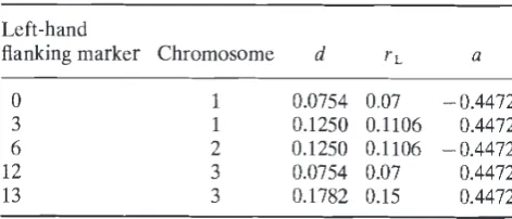
(4) Example
We now give a simple example to show how the methods discussed in this paper might be applied in
practice. A single sample of 2000 F2 individuals was
generated using the genome tabulated in Table 3. This has three chromosomes of length 1 M, each with five evenly spaced markers. Markers are there-fore 25 cM apart, which gives a recombination frac-tion between markers of 0.1967. We have numbered the chromosomes 1, 2 and 3, and the markers are numbered from 0 to 14. Additive QTL were located between markers 0 and 1, 3 and 4, 6 and 7, 12 and 13 and 13 and 14, so that we have three isolated QTL and a pair of nonisolated QTL. Heritability was set to 0.5 and all QTL effects were of equal magnitude, scaled so as to give a phenotypic
vari-ance of 1. The first and third QTL effects were
negative and the remainder positive.The regression of phenotype on all markers for
this data set gives a residual sum of squares of
1238.9, with regression coefficients(0, —0.2966), (1, —0.1422), (2, 0.0221), (3, 0.2209),
(4, 0.1956), (5, —0.0189), (6, —0.1922),
(7, —0.2404), (8,0.0100), (9, 0.0108), (10, —0.0254),
(11, 0.0371), (12, 0.3019), (13, 0.2644),
(14, 0.3370).
This immediately suggests the presence of QTL in
intervals (0,1), (3,4), (6,7), (12,13) and (13,14).
Regressing on these markers gives a RSS of 1240.0
with coefficients
(0, —0.2975), (1, —0.1323), (3, 0.2296), (4, 0.1962),
(6, —0.2047),(7, —0.2377),(12,0.3145), (13,0.2640),
(14, 0.3355). (5)
The small change in RSS suggests that the omitted markers do not flank QTL. Omitting each of the markers 0, 1, 3, 4, 6, 7, 12, 13, 14 from this model in turn results in a considerable increase in RSS. The smallest increase is given by omitting marker 1 to
Table 3 Genome used in simulation
Left-hand
flanking marker Chromosome d
ti
a0 1 0.0754 0.07 —0.4472
3 1 0.1250 0.1106 0.4472
6 2 0.1250 0.1106 —0.4472 12 3 0.0754 0.07 0.4472
13 3 0.1782 0.15 0.4472
d is the distance in cM between the QTL and its left-hand flanking marker, rL the corresponding recombination fraction and a the QTL effect.
(0, —0.3735), (3, 0.1977), (4, 0.1955), (6, —0.2086),
(7, —0.2356), (12,0.3192), (13,0.2598), (14,0.3398).
This difference in RSS is highly significant, so we can conclude that any subset of 0, 1, 3, 4, 6, 7, 12, 13, 14 fits the data signficantly less well than the model including all nine markers. Note also that for the model omitting marker 1, markers 0 and 3 have
opposite sign. We pointed out in the section on
Isolated QTL that the regression coefficients of markers flanking a single QTL must have the same sign, so this suggests that a marker flanking a QTL has been omitted from the model.
We shall now use eqn 5 to map the QTL. QTL in the intervals (0,1), (3,4) and (6,7) are isolated, so from the section on Isolated QTL we can use their
regression coefficients to map the QTL. We get
(0.0720, —0.4413), (0.1030,0.4391), (0.1176, —0.4562) as estimates for the recombination fraction between a QTL and its left-hand flanking marker, respect-ively, markers 0, 3 and 6, and the QTL effect. We know that QTL in intervals (12,13) and (13,14) are not isolated and so we cannot estimate without bias their location and effect: the best we could do would be to obtain the line of locations consistent with
these regression coefficients. Note that treating
these intervals as isolated gives esimates for locationand effect of (0.1022, 0.5965) and (0.1218, 0.6181)
for intervals (12,13) and (13,14), respectively, so the bias caused by ignoring nonisolation is considerable.
In conventional regression mapping, to find
posi-tions for the five suggested QTL would have
required a five-dimensional search using n5 differentcombinations with n positions for each marker. Our
analysis shows that there are many equivalent
models for the nonisolated QTL in intervals (12,13) and (13,14) and that we can map the other three QTL algebraically. This clarfies the identification of
nonisolated QTL and reduces considerably the
computational effort. The example is idealized: we have a small genome, a large population size and a high heritability, and this makes the analysis rather straightforward. The same method is applicable in more complicated cases, although deciding which markers to include in the model obviously becomes much more difficult, particularly if the population size is too small to allow simultaneous estimation of regression coefficients for all markers with reason-able accuracy. Selecting a 'best' subset of varireason-ables to include in a regression is a much studied statis-tical problem; see for example Miller (1990). Here there is a further complication in that the regression coefficients are to be used to obtain estimates of the
underlying parameters, the QTL locations and
effects. This imposes certain restraints on the
subsets of variables that should be considered: for
example, if marker k is included in the model,
marker (k—i) or (k+1) should be also. An excep-tion to this rule might be when markers are fitted as
cof actors to absorb the effect of QTL which,
although too small to be mapped individually,
contribute a significant portion of genetic variance.It should also be noted that there is a particular problem with QTL of small additive effect but large
dominance or epistatic effect, for if we select
markers according to their additive effects such loci may be excluded from the model. Whether this is important depends on context: for marker-assisted selection, for instance, we may only be interested in
additive effects.
Dominance and epistasis
The move from additive to nonadditive QTL has interesting consequences. We consider isolated and nonisolated QTL in turn.
Estimationof dominance and epistasis for isolated
o TL
Wright & Mowers (1994) state that in F2 popula-tions the regression of phenotype on marker-type is unaffected by dominance effects. This is easily seen by considering a single QTL with additive effect a and dominance effect d flanked by markers XL and xR. Then cov(xL, y) = cov(xL, ag+d5), where is
one if g =0and zero otherwise. Hence cov(xL,y) =acov(xL,g)+dcov(XL, )
= acov(xL,g)+d[E(&L)—E(xL)E(5)]
=acov(xL, g),
because P(XL = 1, g =0)
=p(XL —1, g 0), and
QTL MAPPING BY REGRESSING PHENOTYPE ON MARKER-TYPE 29
follows that the regression coefficient of x L is also unaffected by d. The argument clearly extends to any number of loci. It should be stressed that this is
an asymptotic result in the sense that any finite
sample will have, because of chance effects, nonzero covariance between additive and dominance effects.Thus we can estimate the location and additive
effect of QTL by regression on marker-type as in the
section on Isolated QTL and then fit the model
m n
1=1 i=1
to estimate the dominance effects d, because
p (g1 =0Ix), the probability of heterozygosity given
marker-type x, can be calculated given an estimate of the position of the ith QTL. Epistatic effects can
obviously be dealt with in the same way.
This may, however, not be the most efficient
method of mapping nonadditive QTL: we are essen-tially using information about the additive effect to estimate QTL location and then using this estimate of location to estimate dominance effects. Better estimates should be obtained in finite samples by using information about additive and dominance effects together, as in the usual regression mapping
approach to mapping QTL with dominance.
Mappingnonisolated QTL with dominance
Wehave seen that in the absence of dominance or epistasis it is impossible to map nonisolated QTL. It might be expected that with dominance the situation becomes even worse, because we have another para-meter to estimate for each QTL. Surprisingly, this is
not so: in Appendix D we present a method of
mapping two QTL in adjacent intervals when at least one of the QTL has nonzero dominance effect. It follows that the Martinez & Curnow (1992) three marker regression method will work for this situa-tion. It is possible to map nonisolated QTL in the presence of dominance effects because the contribu-tions to the means of the marker groups x_1, x1,
x+1,for x_1 x1, x+1 =1, 0, —1, arising from domi-nance result in those marker groups containing more information about the location of the QTL than is present in the absence of dominance, and this more than offsets the extra parameters that must be
esti-mated. These dominance effects also mean that
E (z Ix) isnow a nonlinear function of x.
We have seen that the regression coefficients f3
are unaffected by dominance effects so that it is only
possible to restrict the position of two QTL in
adja-cent intervals to a line of possible solutions using the
The Genetical Society of Great Britain, Heredity, 77, 23—32.
regression coefficients. Thus it is impossible to add dominance effects to the regression model as we did for isolated QTL in the section on Estimation of dominance and epistasis for isolated QTL. The best we could do would be to fit the model
E(Y)=
+f3+
+d,p(g, =0jx1xj)=01x1x1+i)
for
values of p(g1=OIx1_ix), p(g+i=0x1x+i)
values to find the r_1>, r(+l)l) minimizing the
residual sum of squares. This is equivalent to the usual three marker regression method. A compu-tionally simpler approach would be to fit the addi-tive model to get estimates of I3ji, /3, I3+ and then calculate the RSS for models including dominance terms along the line of QTL locations compatible with these coefficiellts. This has the advantage that we search over one dimension instead of the two
required by Martinez & Curnow, but as in the
section on Estimation of dominance and epistasis for isolated QTL this two-stage process may not make full use of available information. The two
approaches will be identical if and only if the
minimum obtained by the two-dimensional search lies on the line obtained from the regression coeffi-cients of the additive model, and this may not be true in finite populations.
Discussion
We
have presented a method of mapping QTL
based on the regression of phenotype on marker-type. The method removes the need for a numerical search procedure as used in conventional regression mapping and allows unbiased estimates of all isola-ted QTL to be obtained from a single regression. We have assumed that no marker observations are missing, but it should be easy to deal with missing marker observations using the methods of Martinez
& Curnow (1994).
The expression of marker-group means as the sum
of contributions from the right and left flanking
markers is informative in stressing that the QTL we find are really covariances between a marker and
phenotype. There is an infinite number of QTL
configurations that would result in the same marker group means. The fact that we have only enough information to fit one QTL in the interval does not mean that only one QTL exists. In the absence of further information we should perhaps regard the estimated QTL positions as representing the 'centre of gravity' of loci within the interval that affect the
means do not provide sufficient information to map additive, nonisolated QTL. Maximum likelihood methods extract slightly more information from the
data than do regression methods, but produce
almost identical results for isolated QTL. We would expect that this additional information would be sufficient to allow estimates of effect and position for nonisolated QTL but that these estimates would be very imprecise. The situation is analogous with
attempting to map a QTL using single marker
methods: maximum likelihood can in theory esti-mate both position and effect, whereas regression cannot.
We have shown that it is impossible to locate
nonisolated QTL within their intervals. For the same
reasons it may be impossible to distinguish isolated from nonisolated QTL. For example, consider a chromosome in which every other marker interval contains a single QTL, with all the QTL effects having the same sign, say positive: the QTL are therefore isolated and can be mapped. However, all
markers will have positive regression coefficients and
so we cannot tell from the data that the QTL are isolated; the data could equally well come from a number of models, including one in which every interval contains a QTL. To know that a QTL is isolated we require that the marker to the left of the left-hand flanking marker has a regression coeffi-cient which is either of opposite sign to that of the flanking marker or zero, and the marker to the right of the right-hand flanking marker has a regression coefficient which is either of opposite sign to that of
the flanking marker or zero.
These problems may not be important in some applications. In particular, E(z Ix), the expected genetic value conditional on marker-type, depends only on the regression coefficients /3, so that in F2 populations marker-assisted selection (MAS) can be
performed using /3with the same efficiency as if the QTL had been mapped. It should be stressed that this is only true for F2 populations: in subsequent
generations the situation is more complicated,
although it is easy to show that the result holds for
infinite populations in the absence of selection. Also,
computer simulations to compare MAS based on
regression of phenotype on marker-type with a
method more akin to regression mapping showed little difference between the two methods over a 20
generation time span (Whittaker et a!., 1995).
The fact that nonisolated QTL with dominance can be mapped is intriguing, but probably not very useful. A limited amount of computer simulation of QTL with dominance has been performed and this
suggests that although hypothesis tests for the
signif-icance of dominance terms have reasonable power,
the estimates of location obtained are poor. It
should also be noted that, if a dominance effect is included when mapping nonisolated additive QTL, a minimum will be found in the RSS surface because of chance variations in the values of the marker group means. The difficulties of mapping noniso-lated QTL cannot be overemphasized.
Finally, we would expect that epistasis between two nonisolated QTL would allow these QTL to be
mapped in the same way as dominance effects,
although this has not yet been investigated.Acknowledgements
J.C.W. was funded by the BBSRC and P.M.V. by the Marker Assisted Selection Consortium of the
U.K. pig industry (Cotswold Pig Development,
J.S.R. Farms, National Pig Development Company, Newsham Hybrid Pigs, Pig Improvement Company,
and the Meat and Livestock Commision). R.T.
acknowledges support from MAFF. We thank Chris Haley and Robert Curnow for helpful discussions of
this work.
References
EIALDANE, 2. B. s. 1919. The combination of linkage values
and the calculation of distance between loci of linked
factors. .1. Genet., 8, 299—309.
HALEY, C. S. AND KNOTT, S. A. 1992. A simple regression
method for mapping quantitative trait loci in line
crosses using flanking markers. Heredity, 69, 315—324.
JANSEN, R. C. AND STAM, p 1994a. High resolution of quantitative traits into multiple loci via interval
mapping. Genetics, 136, 1447—1455.
JANSEN, R. c. 1994b. Controlling the type I and type II errors in mapping quantitative trait loci. Genetics, 138, 871—881.
LANDER, E. S. AND BOTSTEIN, D. 1988. Mapping Mendelian factors underlying quantitative traits using RFLP
linkage maps. Genetics, 121, 185—199.
MARTINEZ, 0. AND CURNOW, R. N. 1992. Estimating the
locations and the sizes of the effects of quantitative
trait loci using flanking markers. Theoi App!. Genet., 85, 480—488.
MARTiNEZ, 0. AND CURNOW, R. N. 1994. Missing markers when estimating quantitative trait loci using regression mapping. Heredity, 73, 198—206.
MATHER, K. AND JINKS, J. L. 1977. Introduction to
Biome-trical Genetics. Chapman and Hall, London.
MILLER, A. J. 1990. Subset Selection in Regression.
Chapman and Hall, London.
STAM, i'. 1991. Some aspects of QTL analysis. Proceedings
of the Vilith meeting of the Eucarpia Section Biometrics
in Plant Breeding. Brno.
THOMP-QTL MAPPING BY REGRESSING PHENOTYPE ON MARKER-TYPE 31
betweenmarker 1 and QTL 1, by
r
/
41320(1—B)r110.5I 1— 11—
L
\(
[/32+131(1—20)]where 13=2,
132=P1+22 and 133=p2. Supposethat the QTL are of equal effect, a, and that
r11 =r12 r22 =r23=0.1,which implies that 0 =0.18.
Using the usual formulae for 2, p,, we get
= = 22=P2
=
0.49878a and substitution intothe above gives =0.1283. Thus P12 =0.0696 and a= 1.496a.
Note that the bias is considerable,
despite the fact that marker 3 has been fitted as a cof actor.
Appendix
C: mapping nonisolated additiveQTL
We find the minima of the RSS surface supposing that two adjacent intervals both contain QTL, as in the section on Nonisolated QTL. We shall suppose for simplicity that the markers are equally spaced, with 0 the intermarker recombination fraction and
r the recombination fraction between the actual
QTL i and marker j. Then we showed in the same section that any 2, 2i+1, p,, Pi+i satisfying /3 =2,, =Pi+2i+i and13+= Pi+i shouldgive a minimum
of the residual sum of squares surface. Rewriting these equations in terms of recombination fractions and QTL effects we see that any hypothetical pair of QTL with effects a,, a1 and position described by r,(1_l), r(f+l) satisfying
—13_1)rL0_l)(1—ru_1))(l —2r11) —
r(1
—rd) (1 —2riu-1))0(10)
+fi l)r(+l)(J÷l)(l—r(+l)+l)) (1 —2r(+l)J) r(+lf(1 —r(+l,) (1 —2r(j+l)(j÷l))is consistent with /3J_1, f3, /3j+l. Eliminating Tq in the first term on the right-hand side gives
fl_1)rjq_1)(l—rlq_1))(1 —2rj) r4(1 —rq)(l —2r(j_1))
f3_l)rI_l)(1 —r_ ') (1—20)
(0—rI(J_l)) (B—r,(_l))(l —0—r(J_1))
and, calculating the second term by symmetry we get
f3
1—20 SON, R. 1995. Using marker-maps in marker-assisted
selection. Genet. Res., 66, 255—265.
WRIGHT, A. J. AND MOWERS, R. P. 1994. Multiple regression for molecular-marker, quantitative trait data from large
F2 populations. Theor App!. Genet., 89, 305—312.
ZENG, Z.-B. 1994. Precision mapping of quantitative trait loci. Genetics, 136, 1457—1468.
AppendixA: linearity of E(gk'LXR,TL)
As in the section on Expected values of marker-class means,
let 2 =
E(g Jx L =1, X R =0,rL) and
p =E(gJxL =O,XR=1,rL). From Table 1 this is
rR(1—rR)(l—2rL) rL(l—rL)(l—2rR)
2=
andp=
0(1—0) 0(1—0)
so we see immediately that E(gxL= —1, XR=O, rL) = —2and E(gXL =O,XR= 1,rL) = —p.Also,
—TR(l—rR)(l —21L)
+rL(l
rL)(l —2rR)0(1—0)
—rR(l
—rL)(l rRrL) +rL(l —TR)(l rLrR)
—0(1—B)
—l—rL—rR
1—0
=E(gx1,xg=1,rL)=_E(gIXL—l,
XR=
l,rL)
and2—p
TR(l—rR—2rL+2rRrL)—rL(l—rL—2rR+2rRrL)
—(rR_rL)[1_rR(1—rL)—rL(l—TR)]
0(1—0)
=E(gxL=1,xR_1,rL)—E(gIxL=l,
XR = 1, rL)so thatE(gIxL,xR, rL)=AxL+pxR as required.
AppendixB: bias when nonindependence of
QTL is ignored
Suppose
that markers 1 and 2 flank QTL 1 and
markers 2 and 3 flank QTL 2, with no QTL to the left of marker 1 or right of marker 3. Then treating
QTL 1 and 2 as isolated and supposing the recombi-nation fraction between markers 1 and 2 to be 0 we
would estimate r11, the recombination fraction
The Genetical Society of Great Britain, Heredity, 77, 23—32.
1
x [flJrl)(1 —r_i))(0—r(,)U+l))(l —0—r(1!)+1))
+ /3+I)r(+l)+i)(l —rQ+i)&÷i))(O —rl))(l — 9—r1l))].
Writing x =r0_I)(1 —r_I)),y r+l)q+i)(l—r(+l)(j+i))
and simplifying shows that x, y satisfy
o=
+/31+1)JAy
—0(1—0){[/3+/3_((1—2O)Jx+{fl1+/3+i((1—2O)]y}.
Thus,given the regression coefficients /3j-J /3, /3j÷,
the set of possible locations of the two QTL is the
set of r1U_i) E (0,0), r(+i)U+i) E (0,0) satisfying this
equation. This can be easily computed for any /3,
/3
f3+.Appendix D: mapping non isolated QTL with dominance
Again suppose that markers 1 and 2 flank QTL 1 and markers 2 and 3 flank QTL 2, with no QTL to the left of marker 1 or right of marker 3. Let the recombination fraction between QTL i and marker j be r,j,the recombination fraction between markers i and jbe 0,, and the additive and dominance effects of QTL i be a, and d,, respectively. Then we can
write the means of the marker classes as
,
+p1+22+p2+d1+d1for the classx1 1, x2 1, x3 =1+Pi +22+dL +d0 for the classx1 = 1,x2 =1,
x3 0
)1+p1+)2—p2+d1+d_1 for the classx1 =1,
x2=1,x3= —1
and so on,
whered =
d1p(g1 =0lxi = i, x2 =j),d=d2p(g2=0lx2=i,
x3=j) and p(g1=01x1=i,
x2 =1) has
been tabulated in Table 4. Note the
following relations:
Table 4 p(g1 =0lxi =i,x2 =j) for F2 populations
x1 x2 p(g1=01x1=i,x2=j)
1 1 2r11(1 —r11r12(1—r12)/(1 —912)
1 0 r(1 —rn)[1—2ri2(1—r12)I/0i2(1—012)
1 —1 2ri1(1—r11r12(1 —r12)/92
0 1 r12(1 —r12)[1 —2ru(1 —ru)1012(1 —012)
0 0 {[ri+(1_rn)2][r2+(1_ri2)2J}/[92+(i_Oi2)2]
0 1 r12(1 —r12) [1 —2r11(1 —ru)I/012(1 —012)
—1 1 2r11(l —r11r12(1 —r12)/02
—1 0 r11(1 —r13)[1 —2r12(1 —r12)]/012(1—012)
—1 —1 2ru(1—r0r12(1—r12)/(1—012)2
p(g1=0ix1=1,x2=1)=p(gi=0x1=—1,x2=—1)
p(g1= 0 lxi 1,x2 = 1) = (1_012)2p(gi=0 lxi = 1,
x2= —1)
p(g1=01x1=1,x2=—1)=p(g1=01x1=—1,x2=1)
p(gi=0x1=1,x2=0)=p(g1=0lx1= —1,x2=0)
(6)
p(g1=Olx1=0,x2=1)=p(gi=Olx1=0,x2=
—1) We now show that given the 27 marker group meansm,Jk for i, j, and k equal to 0 or 1, it is possible to
map the two QTL, in spite of their
nonindepen-dence. We have
m111 =21+p1+)2+p2+d1+d1
= ______
023
and we know that /3 =), /32 = pi +A2 and /33 =P2 can be found by regression of phenotype on marker-type, because the /1, are independent of the
domi-nance terms. Thus we can find
d1+d1 =m111—/31—f32—/33
d1+
93 2d2 = m0_1—131—/32+133 —023)and subtracting gives
12923d2 =m11_1—m111+2133
023
where the right-hand side is known; hence we can estimate d1, and therefore d1. Similarly, the eqn d1+d1 =m011+132+133 allows d01 to be estimated. From Table 4
d11 — 2012rn(1—r11)
d
(1—012)[1—2r11(1--r11)J'which implies that —2[d
(1 —012) + d 10i2]
r11(1—r11)+d1(1—012) =0, and this quadratic can be solved for r11. Substitution into the appropriate
equations now allows the estimation of r21, a1, a2, d1
and d2. (Note that we need only d1 0 or d2 0 for
this method to work.)
We stress that this is not the optimal method of mapping nonisolated QTL, because it ignores some of the available information. It is presented to show that the means of the marker classes provide suffi-cient information to map nonisolated QTL with
dominance, and that therefore the usual three
marker regression method (Haley & Knott, 1992;
Martinez & Curnow, 1992), which does use all