A PARALLEL SCHEDULING SEQUENCE OF GF (P) EDWARDS COORDINATES COMPUTATION FOR ECC

(1)

ISSN:1992-8645 www.jatit.org E-ISSN:1817-3195

AACGFA : ADAPTING AUTO-CONFIGURATION

GEOGRAPHICAL FIDELITY ALGORITHM FOR MOBILE

WIRELESS SENSOR NETWORKS

1

MBIDA MOHAMED,2DR EZZATI ABDELLAH

1_{Research Scholar., Department of Emerging Technologies Laboratory (LAVETE), Faculty of Sciences}

and Technology Hassan 1st University, Settat, Morocco 2

Professor., Department of Emerging Technologies Laboratory (LAVETE), Faculty of Sciences and Technology Hassan 1st University, Settat, Morocco

E-mail: [email protected],[email protected]

ABSTRACT

Today Mobile Wireless sensor networks (MWSN) are used in several areas. There are many environments of developments and designs MWSN in programing level according to projects needs, however in this article we will design a MWSN model using design tools as Wisen Profile (model devoted to a Driven Development MDD paradigm precisely in Topology of applications) that aims to extend the lifetime of MWSN and have a powerful communication covered network and also provide a number of nodes reachable in case the default path is isolated. We will simulate this new Algorithm of Topology control called AACGFA(Adapting auto-configuration geographical fidelity algorithm), and we proceed to a comparative study with GAFA (geographical adaptive fidelity) algorithm, to see if the AACGFA make more optimal energy consumption and strongest connectivity between nodes .

Keywords: Mobile Wireless Sensor Networks (MWSN), Topology control (TC), Model Driven Development (MDD) , Wisen Profile(WP), geographical adaptive fidelity algorithm( GAFA), Duty Cycle, Feature Model (FM).

1. INTRODUCTION

MWSN presents a collection of a number of sensor nodes where every node is composed with the unit as sensing, transmission and energy control. We can consider it as a embedded system purpose the collection and the relay of data in different domains. Common uses are to detect continuous operation, events, localization and actuate local control actuators . We are going to build and design diverse MWSN entities in order to locate the Topology control (TC) unit . For example of design models in MWSN : the management requirements , The configuration error of MWSN in different situations which can cause fail/loss of the entire network, the behavior of MWSN is highly unpredictable and dynamic. We have to take care of all the factors incorporated by various sensor network models that describe the

current networks state. Some examples of suggested models are:

Network Topology Model: describing the actual topology map and the connectivity and/or reachability of the network. It also may assist routing operations and obtaining information about future deployment of nodes, since the topology of a network affects many of its characteristics, such as latency, capacity, and robustness, as well as the complexity of data routing and processing.

Residual Energy Model: describes the remaining energy level of the nodes or the network. Using this information as well as the data from network topology, coupled together; would make it possible to identify the weak areas (i.e., areas that have short lifetime) of the network

(2)

Usage Patterns Model: represents the activity of

the network in terms of period of time for nodes’

activity, quantity of data transmitted per sensor unit or the movements made by the target, and tracking of hot spots in the network to avoid latency problems.

Behavioral Model: describes the behavior of the network. Since sensor networks are highly unpredictable, dynamic, and unreliable, statistical and probabilistic models may be much more efficient in estimating the network than estimating the network performance than deterministic models. Coverage Area Model: a sensing coverage area

map which represents an actual sensor’s view of the

environment and communications coverage map. Our research requirement focuses on modeling a new Algorithm of TC, with optimized energy consumption combined with higher network performance. The remaining of this paper is organized as follows:

Section 2: present the Model-Driven Development (MDD) paradigm in order to define the TC requirements for conserving energy combined with improved connectivity.

Section 3: Present the proposed feature model(FM) using WSN concepts by integrating the TC entity. Sections 4 and 5: Present the theoretical and experimental views of the GAFA and AACGFA. Section 6: Make a comparative study between the two algorithms to examine which one ensures enhanced connectivity and extending lifetime. Section 7: Conclusions of the research and proposed future work which give a continuity of our studies.

2. RELATED WORK :

In the literature, there are a number of works related to the TC, the most used focused on XTC . XTC is a TC algorithm that works with the mechanism of the links qualities between neighboring nodes [Wattenhofer & Zollinger, 2004].However XTC uses four TC operating properties (symmetry, connectivity, sparseness, and planarity) with a speed performance compared to previous algorithms , and it works also without knowing the location of cooperative nodes whatever the environment.

In communication between nodes , the energy increases quadratically according to the distance to the sink [Wattenhofer & Zollinger, 2004]. XTC also is connected on Euclidean graphs .

XTC has the disadvantages that not apply the multi state service and do not consider node failure and mobility, for this reason, we design two new algorithms (GAFA, AACGFA) that ensures the three functions at once .

3. MODEL -DRIVEN DEVELOPMENT APPROACH (MDD) :

Model-driven development (MDD) is an emerging software development approach that aims to repair the dysfunctions report between the problem area and solution area. Especially, models are operate to build high-level particularizations, and also important for the development mechanism. This is a big advance in the traditional software development steps, however the software design and development are detached. For example of model , all along the software analysis and design step, use cases, interaction diagrams, class diagrams, and other UML diagrams are regularly used to illustrate the problems in order to be solved. However, these artifacts are only comprehensible by people, not by computers. When the coding phase begin, these diagrams pass over because very few people want to return and update the design documents to make them suitable with the software development. The design documents progressively waste their values as the development phases. This tendency cause also other complex, maintenance and documentation problems. As the design documents are always not modified, developers who did not participate in the initial development have a hard time to understand the mechanism by reference to the available documents. Consequently, it is also hard for them to manage the system well.

(3)

code. MWSN needs are typically determined in structural UML diagrams, like a class diagrams. Class diagrams have classes and liaisons used in a specific application. However each WSN application is defined in a diverse class diagram. Moreover, this domain owns mutually exclusive information similarly to technologies used to implement and to deploy a WSN system considering a schedule of hardware and software information (e.g. OS and APIs that map to a different source-code implementation).All the same UML behavior diagrams as sequence confess to represent the common behavior among nodes .

4. MODELING NEEDS USING THE FEATURE MODEL (FM) :

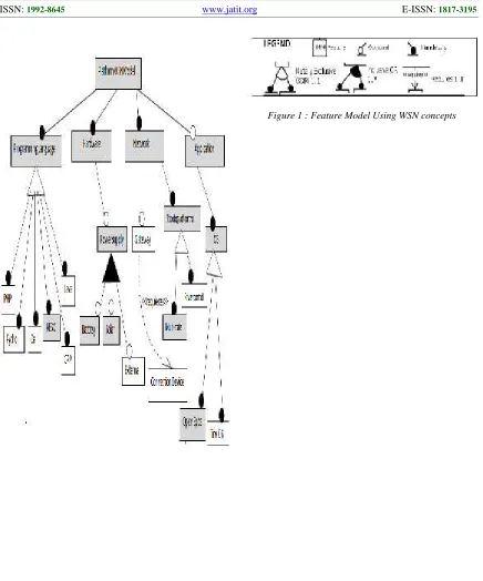
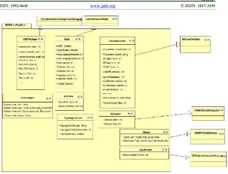
The specific needs and aims in software engineering are identified with the feature model . FM model presents several properties (includes all Functional requirements, architectural, mixed technology ...). Such as it uses can be resumed in the configuration of different needs platform / software. This model defines the different entities of a given technology which aims to establish a communication between platforms variables for MWSN. In the wsn domain, FM gives a different design of services and data control components and networks (TC: topology control in our article) as presented in Figure 1. it is also an interactive model with the change in MWSN applications by domain, which offers the new presentation with the system based on requirements for MWSN .After the identification of systems components , a class diagram is required to capture overall execution values which presents the target application needs (in this case ATP: Application Topology of control) in order to move to the Wisen Profile ( Figure 2 ) that details the stereotypes of MWSN and to better visualize the TC components.

5. GAFA: GEOGRAPHICAL ADAPTIVE FIDELITY ALGORITHM

5.1 Theorical study:

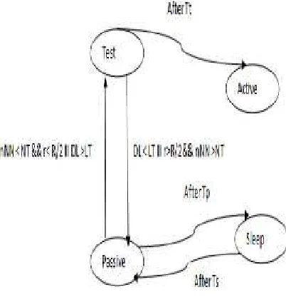
This topology control algorithm have the property to save the energy by changing its status to active nodes or leave unnecessary passive nodes in order to maintain the stability of routing fidelity. This algorithm is mainly based on GPS location and information on the size of each virtual grid, however, each node in the same grid cooperates with its neighbors in order to determine the duty cycle that everyone must apply, this alternative is managed by the system information. Each node in this approach take three states: sleep, discovery or

[image:3.612.317.520.190.447.2]

active as shown in the transition diagram (Figure3). By convention all the nodes of the grid start with the discovery state characterized by the exchange of discovery messages ( id node id grid, estimated node active time (ENAT) and the current status of the node) , in addition, every node in this phase puts a time of discovery td .

Figure 3: Diagram of transition states of GAFA

(4)

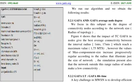
[image:4.612.90.530.71.342.2]

5.2 Experimental GAFA study and analyze: In this section we will establish a simulation of the GAFA in a mobile wsn by using the TC Attariya Simulator which apply the following settings:

Table 1: Parameters of GAF A simulation

We run our algorithm and we obtain the following results:

5.2.1 GAFA AND: GAFA average node degree

We focus in this subpart on the degree of connectivity nodes according to the network size ( Radius of topology ) .

Figure 4 shows that the impact of TC GAFA in nodes give the best average connectivity between the interval radius [ 1mts, 17mts ] which reach a maximum value ( 1,75 MTS) , however the values of Max-componment-size increase progressively regular according to the radius that illustrate just the size of network , the simulation present also that the network outside this range radius of nodes make a low connectivity .

5.2.2 GAFA LT : GAFA life time

A key challenge in MWSN is to develop efficient mechanisms to ensure end-to-end path availability, while incurring minimal control overhead and energy consumption. One of these mechanisms in TC level is the GAFA, in this sub section we will analyze the behavior of the lifetime nodes according to the Covered area of communication and sensing illustrated in the graph (Fig 5):

(5)

6. ADAPTING AUTO-CONFIGURATION GEOGRAPHICAL FIDELITY

ALGORITHM : AACGFA

6.1 Theorical study:

[image:5.612.314.520.134.391.2]

ASCGFA has the aim of exploiting MWSN according to predefined requirements (neighbor threshold, packet loss threshold, maximum radio power....) applied to each node, however it measures the data loss rate (DLR) and the power of radio transmission (PRT), asking the other nodes to join the network and turn on their radio in case of an increase of DLR or PRT lowering, which can be caused by collisions between data packets .

Figure 6: Diagram of AACGFA transactions

In the test phase , the node turn its radio and exchange TC and routings messages , however its own timer Tt is active and the TP/TS ( passive and Sleeping ) timers is off ( Fig 6) .In each duty cycle , ASCGFA node experiment two conditions : the first one is , if the number of active neighbors (nNN )is above the neighbor threshold( NT) , and also if the power radio transmission of nodes is low more than 50% in network , the second event is to test if the average data loss rate (DL) is higher than before entering in test phase (LT), if one of this settings is detected, the algorithm use a contribution of passive list nodes in order to put

the network into the best stability. The next algorithm present this mechanism:

[image:5.612.94.295.311.523.2]

6.2 Experimental AACGFA study and analyze: In this part we evaluate the Average degree and Life time of AACGFA nodes, using by reference the next simulation values:

(6)

6.2.1 AACGFA AND : AACGFA Average node degree

It is useful to analyze the connectivity of nodes in TC in order to see if we can reduce the energy consumption , in our example we run and find the statistics as illustrated in Figure 7.

As shown in Figure 7 the average connectivity take the best value ( 7,5 MTS ) between the radius interval [ 1mts , 17 mts ] , and be approximately null started in 18 mts , on the other hand the Max-componment-size increase with the same progress such as the GAFA-AND graph .

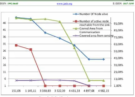
6.2.2 AACGFA LT : AACGFA life time

As indicated in Figure 8 , NNA take a maximum value equal to 50 nodes until a minimum value equal to 15 nodes during the simulation interval, however the NNRS takes a maximum value equal to 50 mts, and decreases until a value of 1 node.

In 4982.15 mts the NNA reach a value of 15 nodes while the NNRS take only one, this occurrence can be explained by the nature of mobility Alive nodes that scattered in the network and become unreachable from the sink. By

reference to the Fig 8 , we see that the CAC reach a maximum value equal to 95% of Covered area at time 1145.11 mts and stay between 65% and 90% along the simulation times , such as the percentage of CAS increase and remain bounded between 5% and 10% for the rest of the simulation .

7. COMPARAISON OF EXPERIMENTAL AACGFA AND GAFA RESULTS :

According to the histogram ( Fig 9) , we found that the average nodes reachable from the sink and the connectivity node degree of AACGFA is approximately double then the GAFA , however the average AACGFA of Covered Area Communication is larger then the GAFA . Moreover the AACGFA give a better performance based on the 3 factors ( NNRS , AND , CAC ) , and the network became more stronger with long life time duration .

7. CONCLUSION:

Various topology of control algorithm are available for deployment in WSNs. TC decides the order in which wireless sensors connect and communicate with each other in a wireless network . In this work, two of TC Algorithms ( GAFA , AACGFA ) were simulated to determine the overall best combination under the simulation constraints and the simulated WSN cases for energy consumption , however we found that the AACGFA give more life time nodes then the GAFA and make a strong connectivity in MWSN . Future work includes the implementation of new design ( CBEMA : cone based and energy management Algorithm ) and make a comparative studies in goal to see if the CBEMA Algorithm is more powerful then AACGFA .

REFRENCES:

[1] L. Mottola and G. P. Picco: Programming wireless sensor networks: Fundamental concepts and state of the art, In: ACM Comput. Surv., vol. 43, no. 3, pp. 19:1- 19:51 (2011)

[2] R. Steiner, T. R. Mück and A. A. Fröhlic: C-MAC: a Configurable Medium Access Control Protocol for Sensor Networks, In: Proceedings of the 9th IEEE Sensors,

pages 845-848, Waikoloa, HI, USA, (2010) [3] B. Bruegge and A. H. Dutoit, Object-Oriented

(7)

Using UML, Patterns and Java, 3rd Edition, Prentice Hall, 2009

[4] J. Fu, F. B. Bastani, and I. Yen, “Automate

AI Planning and CodePattern Based

Code Synthesis”. ICTAI 2006, pp. 540–546. [5] J. Fu, F. B. Bastani, I. Yen, “Model-Driven

Prototyping Based Requirements Elicitation”,

The 14th Proceedings of Monterey Workshop, 2007

[6] J. Fu, V. Ng, F. B. Bastani, and I. Yen,

“Simple and Fast Strong

Cyclic Planning for Fully-Observable

Nondeterministic Planning Problems”,

IJCAI-2011, pp. 1949–1954

[7] A. Gerber, M. Lawley, K. Raymond, J. Steel,

and A. Wood, “Transformation: The Missing Link of MDA”, Proceedings of the 1st

International Conference on Graph Transformation, Barcelona, Spain (2002), pp. 90–105.

[8] A. Kleppe, J. Warmer, and W. Bast, MDA Explained: The ModelDriven Architecture: Practice and Promise. Addison-Wesley, 2003 [9] Michele Zorzi, Wireless Sensor Networks:

Recent Trends and

Research Issues, 4th EURO-NGI Conference on Next Generation

Internet Networks Kraków, Poland, April 28-30, 2008.

[10] Akyildiz,IanF.,etal."survey on sensor

networks." Communications magazine, IEEE 40.8 (2002): 102-114.

[11] Akerberg, Johan, Mikael Gidlund, and M. Bjorkman. "Future research challenges in wireless sensor and actuator networks targeting industrial automation." Industrial Informatics (INDIN), 2011 9th IEEE International Conference on. IEEE, 2011. [12] M. Labrador and P. Wightman, Topology

Control in Wireless

Sensor Networks - With A Companion Simulation Tool for Teaching and Research, Springer Science + Business Media B.V. 2009. ISBN: 978-1-4020-9584-9.

[13] P. Wightman and M. Labrador, “Topology

Maintenance: Extending the Lifetime of

Wireless Sensor Networks,” IEEE LatinCom 2009, September 2009.

[14] P. Wightman and M.. Labrador, “Atarraya:

A Simulation Tool to Teach and Research Topology Control Algorithms for Wireless

Sensor Networks,” ICST 2nd Tools and Techniques, SIMUTools

(8)

[image:8.612.91.527.73.597.2]

(9)

[image:9.612.94.547.70.416.2]

Figure 2 : diagram of proposed wisen profile showing the TC stereotypes

0,00 0,50 1,00 1,50 2,00 2,50 3,00 3,50 4,00

1 2 3 4 18 19 20 31 32 39 40

MaxComponmentSize AverageNodeDegree

[image:9.612.91.542.468.658.2]

(10)

[image:10.612.91.525.70.383.2]

Figure 5 : GAFA LT performance

0,001 1,001 2,001 3,001 4,001 5,001 6,001 7,001 8,001 9,001

1 2 3 4 18 19 20 31 32 39 40

MaxComponentSize AverageNodeDegree

Figure 7 : Average node degree performance

1,00% 11,00% 21,00% 31,00% 41,00% 51,00% 61,00% 71,00% 81,00% 91,00%

1 6 11 16 21 26 31 36 41 46

151,08 1 145,11 3 330,83 3 522,39 4 431,33 4 897,08 4 982,15

Number Of Node alive

Number of active node reachable from the sink Covred Area From Communication

[image:10.612.95.516.432.618.2]

(11)

[image:11.612.90.538.66.359.2]

Figure 8 . AACGFA LT performance

-0,5 1,5 3,5 5,5 7,5 9,5 11,5 13,5 15,5 17,5 19,5

AACGFA GAFA

NNRS AND CAC

[image:11.612.93.533.429.648.2]