BLIND ESTIMATION OF ROOM ACOUSTIC PARAMETERS
FROM SPEECH AND MUSIC SIGNALS
Paul KENDRICK
Built and Human Environment (BuHu)
School of Computing, Science and Engineering
University of Salford, UK
Submitted in Partial Fulfilment of the Requirements of
Table of Contents
Table of figures ... i
List of tables ... viii
Acknowledgments ... xi
Nomenclature ... xii
Abstract ... xv
1 INTRODUCTION ... 1
1.1 Importance of room acoustic parameters ... 1
1.2 Blind estimation of room acoustic parameters ... 2
1.3 Scope, aims and objectives ... 3
1.3.1 Artificial neural network method ... 5
1.3.2 Maximum likelihood method... 6
1.4 Thesis structure ... 7
2 ROOM ACOUSTIC PARAMETERS – DESCRIPTION AND MEASUREMENT METHODS ... 8
2.1 Transfer characteristics of rooms ... 8
2.2 Quantifying the acoustic quality of a room ... 10
2.2.1 The Decay Curve ... 10
2.3 Acoustic parameters ... 11
2.3.1 Reverberation time (Rt) ... 12
2.3.2 Early decay time (EDT) ... 12
2.3.3 Measures of clarity ... 13
2.3.4 Speech transmission index (STI) ... 14
2.3.5 Binaural parameters ... 17
2.1 RIR Measurement methods ... 19
2.1.1 Maximum length sequence measurement ... 20
2.1.2 Swept-sine waves ... 23
2.2 Subjective difference limens ... 23
2.3 Discussion ... 25
3 REVIEW OF EXISTING OCCUPIED ACOUSTIC PARAMETER ESTIMATION METHODS ... 26
3.1 Standard methods at imperceptible levels ... 26
3.2 Model based methods ... 28
3.3 Machine learning based methods ... 29
3.4 Pitch estimation based methods ... 30
3.5 Blind source separation based methods (BSS) ... 31
3.6 Cepstrum based methods ... 31
3.7 Discussion ... 31
4 ACOUSTIC IMPULSE RESPONSE DATABASE ... 32
4.1 Building a database of impulse responses ... 32
4.2 Distribution of sound sources ... 33
4.2.1 Simple geometric room model ... 34
4.2.2 Prediction of acoustic impulse responses ... 37
4.2.3 Simulated impulse response example ... 38
4.3 Distribution of acoustic parameters in the impulse response database . ...41
4.4 Limitations of the database ... 45
4.5 Discussions ... 46
5 OPTIMISATION AND ARTIFICIAL NEURAL NETWORKS ... 48
5.1 Optimisation ... 48
5.1.1 Optimisation overview ... 49
5.1.2 Types of Optimisation algorithms ... 49
5.1.3 Direct search methods ... 50
5.1.4 Gradient search methods ... 51
5.1.5 Simulated Annealing ... 51
5.1.6 Evolutionary Algorithms ... 51
5.1.7 Constrained optimisation ... 52
5.1.1 Choice of algorithm ... 52
5.2 Introduction to Artificial Neural Networks ... 53
5.2.1 The Neuron Model ... 53
5.2.2 Network architecture ... 55
5.2.3 ANN learning algorithms ... 57
5.2.4 ANN applications ... 59
5.3 Discussions ... 60
6 ROOM ACOUSTIC PARAMETER ESTIMATION USING ARTIFICIAL NEURAL NETWORKS ... 61
6.1.1 Envelope Detection ... 63
6.1.2 The ‘Welch’ envelope spectrum detector ... 64
6.2 Data separability ... 65
6.2.1 Mahalanobis distance ... 66
6.3 Training an artificial neural network to estimate room acoustic parameters from reverberated speech ... 67
6.3.1 Training the neural network ... 67
6.3.2 Results using speech signals ... 68
6.3.3 Influence of window width on estimation performance ... 71
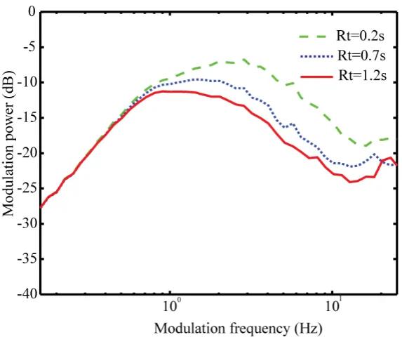
6.4 Effect of reverberation on the envelope spectrum ... 74
6.4.1 Effect of reverberation on the envelope spectrum - summary ... 77
6.5 Training the network to estimate the MTF directly ... 78
6.6 Companding to improve the Rt estimation ... 79
6.7 Estimating room acoustic parameters from reverberated music ... 81
6.8 Problems with music signals ... 82
6.8.1 Envelope spectra of music signals ... 82
6.8.2 Audio spectra of music signals ... 85
6.8.3 The 12th octave filterbank envelope spectrum pre-processor ... 89
6.8.4 ANN estimation results using music signals and the 12th octave envelope spectrum pre-processor ... 90
6.9 Real room impulse response parameter estimation ... 92
6.10 ...Companding music signals to increase Rt performance ... ... 95
6.11 Discussion ... 96
7 IMPROVED MAXIMUM LIKELIHOOD ESTIMATION OF ACOUSTIC PARAMETERS ... 100
7.1 Background ... 100
7.1.1 Determining reverberation time from decay phases ... 101
7.1.2 The Ratnam method for blind estimation of Rt ... 103
7.2 An improved model for sound decay in a room for use in a maximum likelihood framework ... 106
7.2.1 Modelling the decay curve ... 106
7.2.2 Modelling the temporal pattern of received reflections ... 108
7.2.3 A new model of sound decay in a room for MLE ... 110
7.2.4 The maximum likelihood formulation ... 114
7.2.6 Model validation ... 122
7.3 Pre-processing the signal ... 129
7.3.1 Envelope segmentation ... 129
7.3.2 Number of available decay phases ... 132
7.4 Acoustic parameter estimation from ML decay phases ... 132
7.4.1 Method a – minimum Rt ... 134
7.4.2 Method b – global ML estimate ... 141
7.4.3 Method c – optimal estimation of the decay curve ... 145
7.5 Disscussion ... 149
8 APPLICATIONS OF THE MAXIMUM LIKELIHOOD ESTIMATION METHOD .... ...151
8.1 ML Acoustic parameter estimates from speech ... 151
8.1.1 ML Parameter estimates from speech convolved with simulated room impulse responses, 1kHz octave band results ... 152
8.1.2 Results from all octave bands ... 158
8.2 ML parameters from music ... 160
8.2.1 ML parameter estimates from music convolved with simulated room impulse responses, 1 kHz octave band results ... 161
8.2.2 Results from all octave bands (music) ... 166
8.3 Suitability of signals for ML estimation of decay curve ... 172
8.4 Real room measurements ... 173
8.4.1 Distributed RIRs ... 174
8.4.2 ‘The Atrium’ - Bradford University ... 176
8.4.3 The Royal Northern College of Music ... 180
8.5 Maximum likelihood estimation of spatial impression ... 184
8.5.1 Level calibration ... 184
8.5.2 Application of ML to the estimation of ELEF and LG ... 185
8.6 Determining the accuracy of the parameter estimation ... 187
8.7 Performance of the ML method with interfering noise ... 192
8.8 Discussion ... 194
9 IMPROVING THE EARLY SOUND-FIELD ACCURACY USING THE CEPSTRUM ... ... 198
9.1 Limitations of the maximum likelihood method ... 198
9.2 Introduction to the cepstrum ... 199
9.3.1 Detecting echoes using the cepstrum... 204
9.4 Combining the cepstral and ML methods ... 207
9.4.1 Identifying echo locations in the cepstrum ... 208
9.4.2 Assigning levels to detected reflections ... 210
9.4.3 Parameter estimation accuracy using the enhanced ML /cepstrum impulse estimate216 9.4.4 Comparison of the ML and the ML/cepstrum methods ... 217
9.5 Discussion ... 218
10 COMPARISON OF THE ENVELOPE SPECTRUM AND MLE METHODS ... 220
10.1 Speech ... 220
10.1.1 Simulated RIRs ... 220
10.1.2 Real, measured RIRs ... 222
10.2 Music ... 224
10.3 Simulated RIRs ... 224
10.4 Real, measured RIRs ... 226
10.5 Discussion ... 229
11 OVERVIEW, CONCLUSIONS AND FURTHER WORK ... 232
11.1 Overview ... 232
11.1.1 Envelope spectrum method ... 232
11.1.2 Maximum likelihood method ... 234
11.1.3 Comparison of the two methods, implications and accuracy ... 237
11.2 Further work ... 238
APPENDIX ... 242
A. Image source description of sound decay in a room ... 242
B. Acoustic parameter distribution for database of simulated room responses used in ML estimation. ... 242
C. Acoustic parameter distribution for database of real room responses used in ML estimation ... 245
D. Anechoic music pieces ... 248
E. Alternative methodology – training the ANN on the MTFs directly .... 249
F. Additional results – MLE ... 257
i
Table of figures
Figure 2-1. Effect of the room response on a sound source ... 9
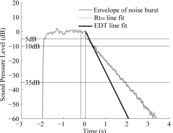
Figure 2-2. Decay curve of an enclosure, the straight lines demonstrate how the Rt30 and EDT are calculated. After Kendrick et al. [9] ... 11
Figure 2-3. Room response to a signal including measurement noise ... 20
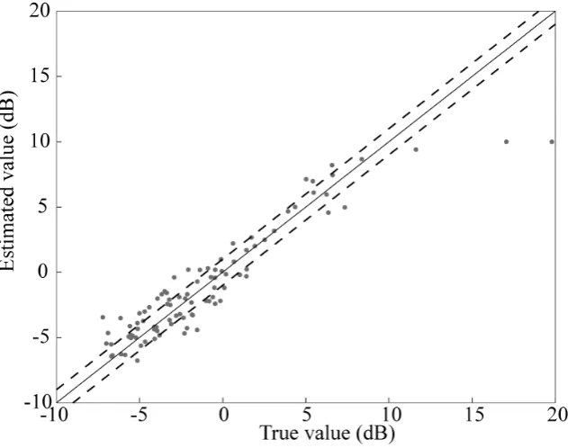
Figure 2-4. Example of plot showing accuracy of C80 estimations. Each dot represents an estimation and the difference limens are represented by dashed lines. This gives an indication of the accuracy of the method ... 25
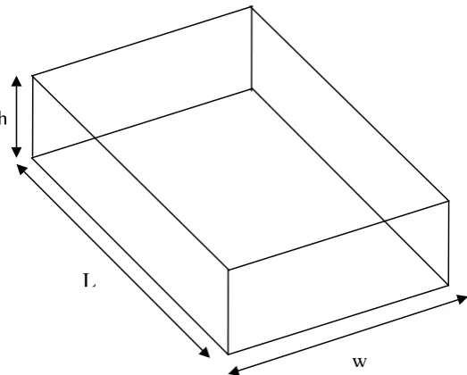
Figure 4-1. Model 1, Box shaped room model. ... 34
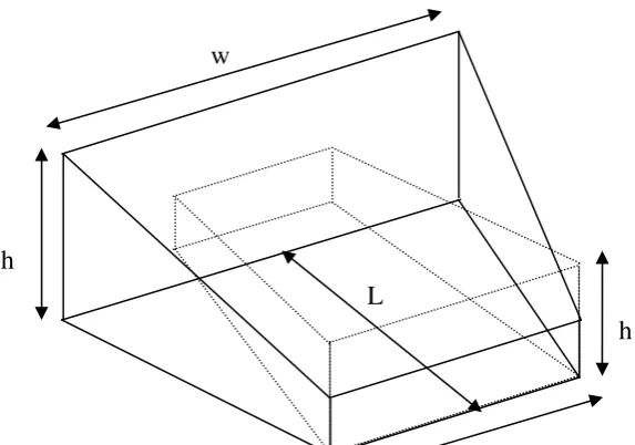
Figure 4-2. Model 2, Fan shaped room model. The dotted shape tries to demonstrate how the geometry may vary, and demonstrates how a sloping floor could occur. ... 35
Figure 4-3. Distribution of possible scattering coefficients used in defining the material properties of the room, each line represents the distribution of possible scattering coefficients used in the room model for each octave band. ... 37
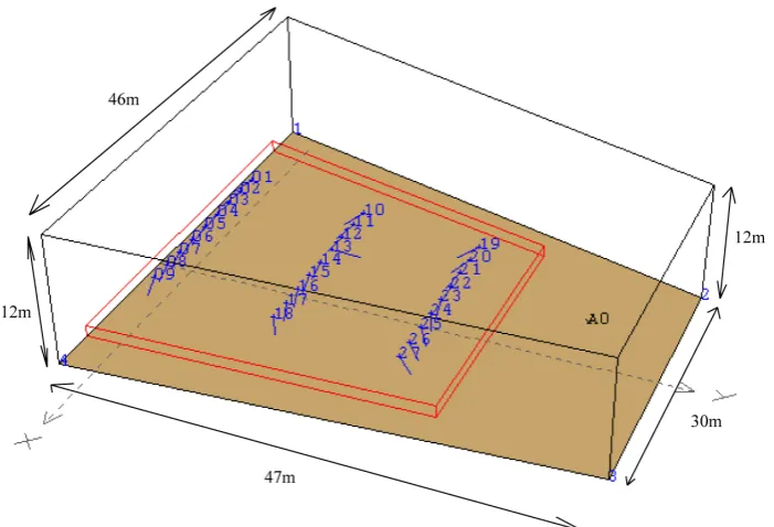
Figure 4-4. View from CATT acoustic showing one of the randomly generated room geometries. The sound source is labelled as A0, the grid of receivers is numbered from 1 to 27. ... 39
Figure 4-5. a) Simulated room impulse response and b) decay curve produced from simulated impulse response for the example room model. ... 41
Figure 4-6. Distribution of Rt and EDT and C80 values in the database of 8400 simulated room impulse responses averaged over the octave bands from 63Hz to 8000Hz. ... 42
Figure 4-7. Distribution of Rt values in the database of 8400 simulated room impulse responses for the octave bands from 63 Hz to 8000 Hz. ... 43
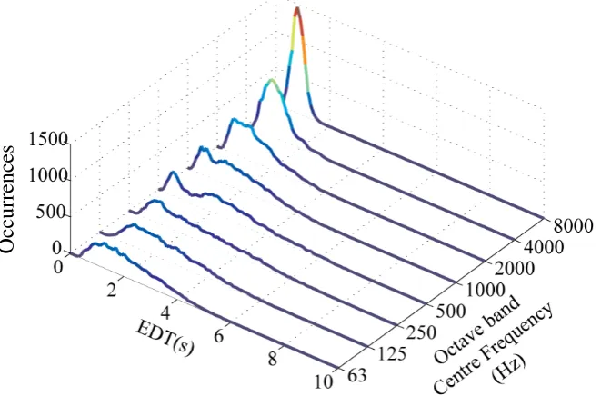
Figure 4-8. Distribution of EDT values in the database of 8400 simulated room impulse responses for the octave bands from 63 Hz to 8000 Hz. ... 43
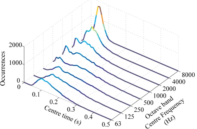
Figure 4-9. Distribution of centre time ts values in the database of 8400 simulated room impulse responses for the octave bands from 63 Hz to 8000 Hz. ... 44
Figure 4-10. Distribution of clarity C80 values in the database of 8400 simulated room impulse responses for the octave bands from 63 Hz to 8000 Hz. ... 44
Figure 5-1. Artificial neuron model ... 54
Figure 5-2. Examples of two types of activation function: 1) threshold activation functions can take one of two values, 2) sigmoid activation functions are continuous. ... 55
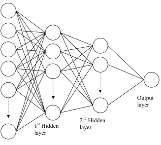
Figure 5-3. Multi-layer feed-forward neural network architecture ... 56
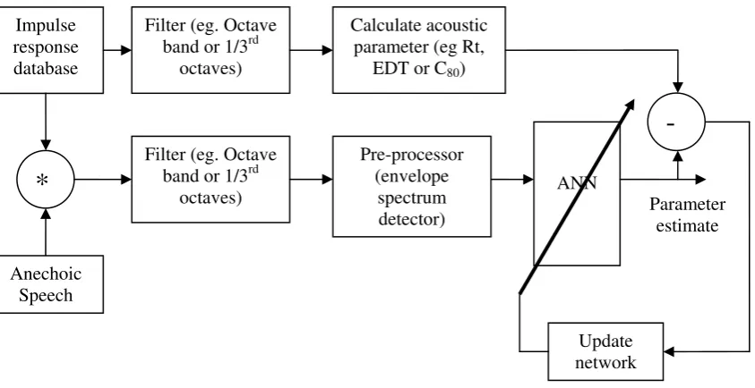
Figure 6-1. Envelope spectrum method - ANN training phase. ... 62
Figure 6-2. Envelope spectrum method - ANN retrieval phase ... 63
ii
Figure 6-4. ANN training phase error showing the error in the training and validation sets. Each epoch
represents a step through all of the data set. ... 69
Figure 6-5. ANN estimation results on test data set for Rt using speech as test signal. Red lines indicate the subjective difference limen. ... 70
Figure 6-6. ANN estimation of EDT, from speech signal, results from test set. ... 71
Figure 6-8. ANN estimation of Clarity from speech signal, results from test set. ... 73
Figure 6-9. ANN estimation of Centre time from speech signals results from test set. ... 74
Figure 6-10. MTF evaluated for a model of non-uniform sound decay using a sum of exponentials. The partial MTFs are shown for each exponential as well as the cross term and the whole MTF ... 77
Figure 6-11. µµµµ-law companding transfer function. ... 80
Figure 6-12. µ-law companding; effect on Rt accuracy. ... 81
Figure 6-13. Envelope spectra of music signals compared with speech envelope spectra, figure legend indicates the piece of music ... 83
Figure 6-14. Data separability as described by the Mahalnobis distance for a sum of sine waves modulating white noise convolved with the RIR database for 1) Rt and 2) EDT. The Mahalnobis distance group step size was 0.1s. ... 85
Figure 6-15. Audio spectra for a selection of the music signals (3&4) and speech in the 1kHz octave band. ... 86
Figure 6-16. Unevenly excited reverberation time compared to the true, evenly excited value. The unevenly excited reverberation time has the same octave band frequency response as a typical piece of music. The dashed lines indicate limits derived from the perceptual difference limens after Kendrick et al. [73]. ... 88
Figure 6-17. Unevenly excited EDT compared to the true, evenly excited value. ... 89
Figure 6-18. Schematic of 12th octave envelope spectrum method for estimating room acoustic parameters from music, after Kendrick et al. [73]. ... 90
Figure 6-19. Variation of the Mahalanobis distance ( ) and envelope spectrum method accuracy (*) with the variance of the music spectrum. 6 pieces of music and one piece of speech(EDT. after Kendrick et al. [73]. ... 92
Figure 6-20. Error in Reverberation time estimation, using set of real room impulse response as test set, dotted lines indicate subjective difference limens. ... 93
Figure 6-21. Error in EDT estimation, using set of real room impulse responses as test set. ... 94
Figure 6-22. Error in ts and C80 estimation, using set of real room impulse responses as test set, dotted lines indicate subjective difference limens. ... 95
iii
Figure 7-2. Histogram of ML decay curve estimates, showing order statistics method of choosing Rt estimate. ... 104 Figure 7-3. Histogram of ML decay rate estimates, showing how the first peak is selected as the best
estimate. ... 105 Figure 7-4. A room impulse response showing the increase in reflection density with time. ... 109 Figure 7-5. This figure shows an example of the RIR model generated from the above parameters. The
plots show both the estimated envelope of the RIR (in red) and the RIR estimate (in blue) ... 111 Figure 7-6. Schroeder curve of room impulse response models, the backwards integrated impulse
response model and the backwards integrated RIR envelope are shown to be similar. a) shows the full dynamic range of the decay while b) shows a small section highlighting the random fluctuations in the impulse response model. ... 112 Figure 7-7. A dual exponential decay model can give non-uniform decay, where the faster decaying
exponential dominates the early part of the decay curve, and the slower decaying exponential controls the late part of the decay. The decay envelopes for three different weighting factors as shown in the legend are illustrated. ... 114 Figure 7-8. The likelihood function over a grid of exponential parameters a2 and a1. At each location
the solution has been optimised with respect to the parameter; αααα. The maxima represent the local and global solutions. The bottom plot is a magnification of a section of the top plot as indicated. ... 118 Figure 7-9. Minimisation overview. A two stage algorithm is employed. First a coarse search is
applied to the likelihood function with the aim of finding the region where the global minimum is most likely to be present. Then these parameters are used as the starting point for a more detailed optimization. ... 119 Figure 7-10. The likelihood across a grid of α parameters but with parameters a2 and a1 are fixed. This
clearly shows the smoothness of the function and the single maximum for the α parameter. ... 120 Figure 7-11. Coarse search method. Only the shaded cells are processed due to symmetry, the cost
function is exhaustively computed at all highlighted grid points to reduce the chance of missing out on possible solutions in the coarse search. The sequential quadratic programming method [83] is used to minimize with respect to α at each grid position.121 Figure 7-12. Comparison of dual and single exponential model estimations of Rt (a) and EDT (b).
Maximum likelihood estimation performed directly on simulated room impulse responses. Dotted lines show perception difference limens. ... 123 Figure 7-13. Comparison of the estimated decay curves for an artificial room response using the new
dual exponential model and the single exponential model. ... 124 Figure 7-14. Comparison of the clarity estimated directly from impulse responses using MLE (2s
iv
Figure 7-15. Comparison of the centre time estimated directly from impulse responses using MLE (2s length) vs. the true value ... 126 Figure 7-16. Comparison of the estimated parameters a) Late lateral strength and b) early lateral
energy fraction. (estimated directly on 2s length of artificial impulses using omni and figure-of-8 microphones) ... 128 Figure 7-17. Segmentation with least mean square line fitting to identify free decay phases for further
MLE. (a) Frame with positive k indicating rise edge is discarded; (b) & (c) consecutive frames with negative k are retained to form the decay phase for MLE. (d) Selected decay phases by the heuristic method. After Kendrick et al. [9] ... 131 Figure 7-18. Selected decay phases for a 10s segment of reverberated music. ... 132 Figure 7-20. Probability distribution of maximum likelihood estimates with >25dB dynamic range of
(a) Rt and (b) EDT, compared with actual Rt and EDT values . Minimum ML estimates RTEST and EDTEST are show on the plots. 90s speech stimulus for a single artificial room response. ... 136 Figure 7-21. Comparison of (a) reverberation time and (b) EDT, estimated using multi-decay maximum
likelihood estimation and the true values. Artificially reverberated speech using simulated impulse responses (1 kHz octave band). ... 138 Figure 7-22. Comparison of (a) reverberation time and (b) EDT, estimated using multi-decay maximum
likelihood estimation and the true value. Speech received in real rooms. ... 139 Figure 7-23. Comparison of (a) Centre time and (b) C80, estimated using multi-decay maximum
likelihood estimation and the true value. Speech received in simulated rooms. ... 140 Figure 7-24. Comparison of reverberation time and EDT, estimated using all decay phases with >25dB
dynamic range in a single maximum likelihood estimation and the true value. Speech received in real rooms. ... 142 Figure 7-25. Comparison of reverberation time and EDT, estimated using all decay phases with >25dB
dynamic range in a single maximum likelihood estimation and the true value. Speech received in artificial rooms. ... 143 Figure 7-26. Comparison of reverberation time and EDT, estimated using 180s of speech, reverberated
and segmented into 4 segments. Fastest decaying reponse with at least 25dB dynamic range selected and 4 decay phases used to estimate final decay curve. a) simulated rooms, b) real rooms ... 144 Figure 7-27. Optimal RIR envelope construction from a set of ML estimates. After Kendrick et al. [7]...
...147 Figure 7-28. Optimal Schroeder curve estimation using eight, 60s segments of anechoic speech
convolved with a real RIR. Each decay curve estimate has been backwards integrated to produce a Schroeder curve.[10] ... 149 Figure 8-1. Rt estimated using ML method plotted against the true Rt for 100 simulated impulse
v
Figure 8-2. EDT estimated using ML method plotted against the true EDT for 100 simulated impulse responses and speech. ... 154 Figure 8-3. Comparison of the envelope of the reverberant decay when the RIR is excited using
impulsive excitation and when the response is a sustained noise source switched off after a long period of time. ... 155 Figure 8-4. EDT estimated using ML method plotted against the true EDT. 100 impulses were chosen
at random from a database. Each impulse response was convolved with 9 minutes of speech. For the ML estimation, the reverberated signal was windowed into three, three minute segments. ... 156 Figure 8-5. C80 estimated using ML method plotted against the true C80. 100 impulse responses were
chosen at random from a database. Each impulse response was convolved with 9 minutes of speech. For the ML estimation, the reverberated signal was windowed into three, 3 minute segments. ... 157 Figure 8-6. ts estimated using ML method plotted against the true ts. 100 impulse responses were
chosen at random from a database. Each impulse response was convolved with 9 minutes of speech. For the ML estimation, the reverberated signal was windowed into three, 3 minute segments. ... 157 Figure 8-7. The average error for Rt and EDT as a function of octave band (left plot) and the
percentage of Rt and EDT predicted parameters within the subjective DL (right plot) using simulated impulse responses convolved with 9 mins of anechoic speech windowed into three, 3 minute segments. ... 159 Figure 8-8. Comparison of estimated and true reverberation time. Estimates were obtained from the
application of the ML method to simulated impulse responses convolved with 40 mins of anechoic music windowed into eight, five minute segments. ... 162 Figure 8-9. Comparison of estimated and true reverberation time. Estimates were obtained from the
application of the ML method to simulated impulse responses convolved with 40 mins of anechoic music windowed into 20, two minute segments, results presented. ... 163 Figure 8-10. Comparison of estimated and true EDT. Estimates were obtained from the application of
the MP method to simulated impulse responses convolved with 40 mins of anechoic music windowed into eight, five minute segments. ... 164 Figure 8-11. Comparison of estimated and true EDT. Estimates were obtained from the application of
the MP method to simulated impulse responses convolved with 40 minutes of anechoic music windowed into four, ten minute segments. ... 165 Figure 8-12. Comparison of estimated and true C80. Estimates were obtained from the application of
the ML method to simulated impulse responses convolved with 40 mins of anechoic music windowed into 10 minute segments. ... 166 Figure 8-13. Comparison of estimated and true ts. Estimates were obtained from the application of
vi
Figure 8-15. Noise vs. signal level for anechoic recordings ... 170 Figure 8-16. The selected decay phase estimated from 60s of narrated speech. after Kendrick et al.
[73]. ... 172 Figure 8-17. Examples of the ‘distributed source’ impulse responses. Impulse responses recorded by
orchestra members clapping simultaneously. ... 176 Figure 8-18. Photographs of the Atrium at the University of Bradford. ... 177 Figure 8-19. Decay curve estimates for the Atrium at the University of Bradford. Green lines are
individual segment estimates, red is the optimal decay curve estimate and blue is the averaged true decay curve from four snare hits. Measured at two microphone positions (one and two). ... 178 Figure 8-20. The Haden Freeman Concert Hall, at the Royal Northern College of Music. ... 180 Figure 8-21. Decay curve estimates for the Haden Freeman Concert Hall. Green lines are individual
segment estimates, red is the optimal decay curve estimate and blue is the averaged true decay curve from 4 snare hits. 8, 10 minute segments were used. ... 181 Figure 8-22. Maximum likelihood estimates for a) Early Lateral Energy Fraction (ELEF) and b)Late
Lateral Reflection Strength LG. ... 186 Figure 8-23. Approximate distribution of decay curve estimates, the white line is the median decay
curve ... 189 Figure 8-24. 90% confidence bounds for median decay curve estimation ... 190 Figure 8-25. The 90% confidence limits expressed as a fraction of the actual parameter and averaged
over all parameters, as a function of the segment length. ... 191 Figure 8-26. Effect of change of signal to noise ratio on parameter estimation accuracy using speech as
excitation signal a) result for RT, b) result for EDT. ... 193 Figure 8-27. Effect of change of signal to noise ratio on parameter estimation accuracy using speech as
excitation signal 1) C80 2) ts ... 194 Figure 9-1. Frequency and phase response of the Butterworth filter discussed in the text ... 202 Figure 9-4. Selection of speech utterance onsets, the 500ms sections of speech onsets are highlighted
in red ... 206 Figure 9-5. Estimated early sound field using averaged cepstra from 500ms windows whose starting
point is automatically detected as the initial onsets of speech utterances (a) and averaged cepstra from all 90s of speech using 95% overlapping 3sec windows (b). Plots have been scaled for comparison purpose. ... 207 Figure 9-6. Estimated impulse response using the cepstral method with overall decaying trend
vii
Figure 9-11. Magnitude of the impulse response estimated using combined cepstrum/ML method (a) and true impulse response (b) ... 214 Figure 9-12. Impulse response estimated from reverberant speech using combined cepstrum and ML
method. ... 215 Figure 10-1. Error in parameter estimation versus the true value for reverberation time. The dotted
lines indicate the difference limens. •••• MLE and ο envelope spectrum method. Validation set using simulated impulse responses and speech excitation. After Kendrick et al. [9].221 Figure 10-2. Error in parameter estimation versus the true value for clarity •••• MLE and ο envelope spectrum method. Validation set using simulated impulse responses. Speech excitation. After Kendrick et al. [9]. ... 222 Figure 10-3. Error in parameter estimation versus the true value for Rt. •••• MLE and ο envelope
spectrum method. Validation set using real RIR. After Kendrick et al. [9]. ... 223 Figure 10-4. Error in parameter estimation versus the true value for clarity. ••••MLE and ο envelope
spectrum method. Validation set using real RIRs. After Kendrick et al. [9]. ... 224 Figure 10-5. Error in reverberation time estimation versus the true value. The ••••MLE and ο envelope
spectrum method. Validation set using simulated impulse responses. Music excitation. After Kendrick et al. [9]. ... 225 Figure 10-6. Error in parameter estimation versus the true value: (A) EDT, (B) centre time and (C)
clarity •••• MLE and ο envelope spectrum method. Validation set using simulated impulse responses. Music excitation. After Kendrick et al. [9]. ... 226 Figure 10-7. Error in reverberation time estimation versus the true value ••••MLE and ο envelope
spectrum method. Validation set using real room measurements. Music excitation. After Kendrick et al. [9]. ... 227 Figure 10-8. Error in parameter estimation versus the true value: (A) EDT, (B) centre time and (C)
clarity. •••• MLE and ο envelope spectrum method. Validation set using real room measurements. Music excitation. After Kendrick et al. [9]. ... 228 Figure A.1. Distribution of Rt values for database of 100 simulated room impulse responses for the
octave bands from 63Hz to 8000Hz. ... 243 Figure B-2. Distribution of EDT values for database of 100 simulated room impulse responses for the
octave bands from 63Hz to 8000Hz. ... 243 Figure B-3. Distribution of C80 values for database of 100 simulated room impulse responses for the
octave bands from 63Hz to 8000Hz. ... 244 Figure B-4. Distribution of ts values for database of 100 simulated room impulse responses for the
octave bands from 63Hz to 8000Hz. ... 244 Figure B-5. Distribution of D values for database of 100 simulated room impulse responses for the
octave bands from 63Hz to 8000Hz. ... 245 Figure C-6. Distribution of Rt values for database of 18 real room impulse responses for the octave
viii
Figure C-7. Distribution of EDT values for database of 18 real room impulse responses for the octave
bands from 63Hz to 8000Hz. ... 246
Figure C-8. Distribution of C80 values for database of 18 real room impulse responses for the octave bands from 63Hz to 8000Hz. ... 247
Figure C-9. Distribution of ts values for database of 18 real room impulse responses for the octave bands from 63Hz to 8000Hz. ... 247
Figure C-10. Distribution of D values for database of 18 real room impulse responses for the octave bands from 63Hz to 8000Hz. ... 248
Figure E-11. Neural network method to estimate MTF directly from envelope spectra ... 250
Figure E-12. ANN estimates of MTFs when presented with envelope spectra of reverberant music signal, dotted lines show the true MTF while the bold lines show the estimates ... 251
Figure E-13. Backwards integrated decay curve estimates calculated from MTFs estimated by the ANN method, dotted lines shows the estimates while bold lines show the true MTF. ... 253
Figure E-14. Backwards integrated decay curve estimates(2) calculated from MTFs(1) estimated by the ANN method using PCA pre-processing, dotted lines shows the estimates while bold lines show the true MTF. ... 255
Figure E-15. Estimation of EDT(1) and Rt(2) from PCA pre-processed signals using an ANN with two hidden layers to estimate MTF ... 256
Figure F-16. Real impulse responses 9 mins of speech windowed into 1 ½ minute segments, results presented are for Rt(a) and EDT (b). ... 257
Figure F-17. Real impulse responses, 9 mins of speech windowed into 1 ½ minute segments, results presented are for C80 (a) and ts(b). ... 257
Figure F-18. Real impulse responses 40 mins of speech windowed into 4 minute segments, results presented are for Rt (a) and EDT (b). ... 259
Figure F-19. Real impulse responses, 40 mins of speech windowed into 4 minute segments, results presented are for C80 (a) and ts (b). ... 259
List of tables
Table 2-1. Difference limens for acoustic parameters used in this thesis ... 24Table 4-1. Geometrical constraints imposed on room shapes, geometry must fall within all of these bounds to be classed as valid. Constraints developed pragmatically by considering typical room sizes in the built environment. ... 36
Table 4-2. Surface properties for the room model shown in Figure 3-3, please note 8k and 16k bands are extrapolated from the 2 and 4 kHz octave bands in the CATT software ... 40
Table 4-3. Acoustic parameters for the simulated room ... 41
Table 4-4. Range of parameters seen in concert halls ... 41
Table 5-1. Determining the Number of Hidden Layers, replicated from [63]. ... 57
ix
Table 6-3. Test signals generated for modulators, each modulator is a sum of sine signals, the frequencies of which are listed. ... 84 Table 6-4. Results from training the ANN on music signals using the modified envelope spectrum pre-processor. ... 91 Table 6-5. Companding music signals, comparison of the percentage of results within the DL with and
without companding, results generated from a single piece of music, ANN training was repeated 10 times and the resulting performance indicator averaged. ... 96 Table 8-1. Sampling frequencies chosen for each octave band ... 158 Table 8-2. Summary of the percentage of the predicted room impulse response parameters that are
within one difference limens. Estimates are based on an ML analysis of simulated room responses convolved with 9 mins of anechoic speech split into 3 segments. Results are shown for all octave bands. ... 159 Table 8-4. Summary of the percentage of the parameter estimates that are within a difference limens
of the true value . Estimates are based on an ML analysis of simulated room responses convolved with 40 minutes of anechoic music split into eight, five minute segments for Rt, and four, ten minute segments for EDT, C80 and ts. ... 168 Table 8-6. Average number of decay phases per minute exhibiting at least 25dB of decay, and
percentage of quiet in each anechoic signal. Percentage of quiet is calculated by computing the percentage of (non-overlapping) 0.05s length windows in each signal with energy 40dB less than the maximum energy, after Kendrick et al. [73]. ... 173 Table 8-.7 Comparisons of estimated and true acoustic parameters for ‘The Atrium’ at the University
of Bradford. Estimated parameters were obtained by the ML method while true parameters were obtained from repeated snare hits (parameters were averaged across four responses). ... 179 Table 8-8. Confidence limits on parameter estimates for the acoustic characteristics of the Atrium in
Bradford using the ML method. ... 180 Table 8-9. Confidence limits on parameters computed from the snare drum excited RIR in the Atrium
in Bradford, computed from 4 snare drum hits. ... 180 Table 8-10. Comparisons of estimated and true room response parameters for the Haden Freeman
Concert Hall. Estimated parameters were obtained by the ML method, while true parameters were obtained from hand claps. Actual parameters were calculated from both the 1st violinist’s hand clap but also the whole orchestra clapping simultaneously (parameters were average across a number of responses). ... 182 Table 8-11. Confidence limits on parameter estimates for the acoustic characteristics of the Haden
Freeman Concert Hall in RNCM using the ML method. ... 183 Table 8-12. Confidence limits on parameters computed from the Haden Freeman Concert Hall RIR
x
Table 8-13. Confidence limits on parameter estimates for the acoustic characteristics of the Atrium in Bradford using the ML method. ... 190 Table 9-1. Comparison of averaged absolute parameter error for 100 simulated room impulses
responses comparing the ML method with the hybrid ML+cepstrum method. ... 217 Table 9-2. Comparison of averaged absolute parameter error for 18 real room impulses responses
comparing the ML method with the hybrid ML+cepstrum method. ... 217 Table 9-3. Comparison of the mean square difference between the magnitude of the true impulse and
the magnitude of the two impulse estimates (ML and ML+cepstrum) calculated from 100 artificially simulated impulse estimates. ... 218 Table 10-1. Standard errors for parameters when estimated using the Maximum Likelihood and
envelope spectrum method. Standard errors calculated using simulated impulse responses where Rt<5s. ... 230 Table D-1. Denon anechoic orchestral music recording ... 248 Table D-2. Anechoic recordings of symphonic music; Helsinki University of Technology for more
information. ... 249 Table F-3. Percentage of estimates within difference limens from 9 mins of anechoic speech split into
7 segments. Results are shown for all octave bands. ... 258 Table F-4. Average parameter error from decay curve estimates yielded from 9 mins of anechoic
speech split into 7 segments. Results are shown for all octave bands. ... 258 Table F-5. Percentage of ML parameter estimate from 40 mins of anechoic music segmented into 8, 5
min segments, the music has been convolved with real room impulse responses. ... 260 Table F-6. 95% confidence bounds on ML parameter estimate from 40 mins of anechoic music
xi
Acknowledgments
I am deeply indebted to my supervisor Prof. Trevor Cox for his guidance and excellent
supervision throughout the duration of this project. Throughout our regular meetings he
provided with me with the support and most importantly the encouragement that has
enabled me to complete this research. I am also grateful to my co-supervisor Dr Francis
Li for his invaluable guidance and support. I would welcome any opportunities that
may arise in future to once again work with both Prof. Cox and Dr. Li.
This project was performed in conjunction with the University of Cardiff Centre for
Digital Signal Processing, where Dr Yonggang Zhang and his supervisor Prof. Jonathon
Chambers carried out a concurrent research project, utilising blind source separation
techniques to perform blind estimation of acoustic parameters. The team at Cardiff
were responsible for the development of the envelope segmentation algorithm used
within this thesis. I am grateful to the team at Cardiff for offering their expertise, advice
and support during a number meetings and correspondences.
A number of in-situ orchestral measurements were carried out and thanks go to
Margaret Barry, Head of Orchestras and Ensembles at the Royal Northern College of
Music, and to Mark Robinson, Artistic Director & Fellow in Music the University of
Bradford for allowing me to record and perform measurements during rehearsals.
Thanks also go to Henrik Möller for supplying the real room impulse responses.
I am extremely thankful for the help and support I received from my parents and my
friends, in particular my dad, Dr. John Kendrick, for his help with proof reading and the
occasional seemingly intractable maths problem. I must also thank my sister, Dr. Emma
Kendrick and my mum, Helen Winthorpe Kendrick for offering their proof reading
skills on the final draft. I must also thank my partner Laura for putting up with the
many late nights and frustrations caused by particular problems I encountered.
I would also like to acknowledge the support of the Engineering and Physical Sciences
xii
Nomenclature
Abbreviations
ANN Artificial Neural Network
BSS Blind Source Seperation
C80 Clarity Index
D Definition/Deutlichkeit
EDT Early Decay Time
ELEF Early Lateral Energy Fraction
FIR Finite Impulse Response (filter)
HMM Hidden Markov Model
Hz Hertz
IACC Inter-Aural Cross-Correlation
LG Late Lateral Strength
MLE Maximum Likelihood Estimation
MTF Modulation Transfer function
PCA Principal Components Analysis
RIR Room Impulse Response
Rt Reverberation Time
RTF Room Transfer Response
RMS Root Mean Square
SPL Sound Pressure Level
STI Speech Transmission index
ts Centre Time
LTI Linear Time Invariant
dB Decibel
ASW Apparent Source Width
LEV Listener EnVelopment
G Strength
MLS Maximum Length Sequence
IRS Inverse-Repeat Sequences
JND Just Noticeable Differences
JNND Just Not Noticeable Differences
DL Difference Limens
CMTF Complex Modulation Transfer Function
CD Compact Disk
p(x) Probability density function
tmixing Mixing time
w.r.t with respect to
ML Maximum Likelihood
xiii
Symbols
f(u) Activation function
x(t) Anechoic source signal
ω Angular frequency
Ini ANN input
Outi ANN output
Sxx(f) Auto power spectrum density
log Base 10 logarithm
C1,2 Covariance matrix
CR Cramér–Rao
Sxy(f) Cross Power Spectrum Density
d(t) Decay curve
δ() Delta function
env(t) Envelope of signal
E[] Expected value
τ Exponential time constant
f Frequency
H[] Hilbert transform
yh(t) Hilbert transform of signal
η Learning rate
L() Likelihood function
lnL() Log likelihood function
Dm Mahalanobis distance
µ Mean
θ Model parameter vector
ln Natural logarithm
bi Neuron bias
wi Neuron weight
n(t) Noise signal
y(t) Received signal
Y(f) Received signal Fourier transform
h(t) Room Impulse response
H(f) Room Transfer Function
Fs Sampling frequency
sign(x) Sign of x
X(f) Transmitted signal Fourier transform
σ2 Variance
V Volume
F(x) µ-law transfer function
xiv
“I see the parts but not the whole, I study saints and scholars both,
No perfect plan unfurls, Do I trust my heart or just my mind, Why is truth so hard to find in this world.”
xv
Abstract
The acoustic character of a space is often quantified using objective room acoustic
parameters. The measurement of these parameters is difficult in occupied conditions
and thus measurements are usually performed when the space is un-occupied. This is
despite the knowledge that occupancy can impact significantly on the measured
parameter value. Within this thesis new methods are developed by which naturalistic
signals such as speech and music can be used to perform acoustic parameter
measurement. Adoption of naturalistic signals enables passive measurement during
orchestral performances and spoken announcements, thus facilitating easy in-situ
measurement.
Two methods are described within this work; (1) a method utilising artificial neural
networks where a network is taught to recognise acoustic parameters from received,
reverberated signals and (2) a method based on the maximum likelihood estimation of
the decay curve of the room from which parameters are then calculated.
(1) The development of the neural network method focuses on a new pre-processor
for use with music signals. The pre-processor utilises a narrow band filter bank with
centre frequencies chosen based on the equal temperament scale. The success of a
machine learning method is linked to the quality of the training data and therefore
realistic acoustic simulation algorithms were used to generate a large database of room
impulse responses. Room models were defined with realistic randomly generated
geometries and surface properties; these models were then used to predict the room
impulse responses.
(2) In the second approach, a statistical model of the decay of sound in a room was
further developed. This model uses a maximum likelihood (ML) framework to yield a
number of decay curve estimates from a received reverberant signal. The success of the
method depends on a number of stages developed for the algorithm; (a) a pre-processor
to select appropriate decay phases for estimation purposes, (b) a rigorous optimisation
algorithm to ensure the correct maximum likelihood estimate is found and (c) a method
to yield a single optimum decay curve estimate from which the parameters are
xvi
The ANN and ML methods were tested using orchestral music and speech signals. The
ANN method tended to perform well when estimating the early decay time (EDT), for
speech and music signals the error was within the subjective difference limens.
However, accuracy was reduced for the reverberation time (Rt) and other parameters.
By contrast the ML method performed well for Rt with results for both speech and
music within the difference limens for reasonable (<4s) reverberation time. In addition
reasonable accuracy was found for EDT, Clarity (C80), Centre time (Ts) and Deutichkeit
(D). The ML method is also capable of producing accurate estimates of the binaural
parameters Early Lateral Energy Fraction (LEF) and the late lateral strength (LG).
A number of real world measurements were carried out in concert halls where the ML
accuracy was shown to be sufficient for most parameters. The ML method has the
advantage over the ANN method due to its truly blind nature (the ANN method requires
a period of learning and is therefore semi-blind). The ML method uses gaps of silence
between notes or utterances, when these silence regions are not present the method does
not produce an estimate. Accurate estimation requires a long recording (hours of music
or many minutes of speech) to ensure that at least some silent regions are present. This
thesis shows that, given a sufficiently long recording, accurate estimates of many
acoustic parameters can be obtained directly from speech and music.
Further extensions to the ML method detailed in this thesis combine the ML estimated
decay curve with cepstral methods which detect the locations of early reflections. This
Chapter 1 : Introduction 1
1
INTRODUCTION
The acoustical character of a room is very important in many situations. Acoustical
properties which can enhance speech intelligibility are desirable in lecture theatres and
classrooms. In concert halls and opera houses, acoustics which enhance the listening
experience are highly prized. In factories or train stations, the goal is to have acoustics
that help control the overall noise level and aid speech intelligibility of public
announcements. The lay listener regularly makes judgments regarding the acoustic
quality of a space. In the case of speech the judgments are based on the ease of
understanding the speaker. For music the judgments are much more subjective and
often limited to descriptions of ‘good’ or ‘bad’ acoustics. Although, when pressed, the
lay listener often cannot define what is meant by good or bad acoustics, many studies
have identified particular features in the acoustics of the room that are preferred or
disliked by the general public. By being mindful of particular features of a room that
cause bad acoustics and focusing on features that are preferred, a room can be designed
to be good acoustically. It requires extensive knowledge and experience to predict the
effect that the geometry and materials will have on the acoustics. More recently,
reasonably accurate computer models have been employed to predict the room response,
so that the acoustical properties can be predicted before building commences. These
computer models enable auralisations of the room to be made so the acoustics of the
space may be experienced prior to building. One of the biggest challenges for the
designer of an acoustic space is how to marry the understanding of physical acoustics,
i.e. the behaviour of sound in an enclosed space, with the understanding of the
subjective perception of the acoustics by a listener. In many ways this means the
acoustic designer must be part scientist and part craftsman.
1.1
Importance of room acoustic parameters
The subjective impression of room acoustics is largely determined by the reflections
that are created when a sound source is activated in a room. Particular aspects of the
subjective impression are related to the different properties these reflections may have,
such as the rate of the decay of reflections, the direction of the incoming reflections with
Chapter 1 : Introduction 2
design an acoustic space, particular subjective aspects of room acoustics must be
identified and related to the physical acoustics properties. To achieve this, many
listening tests have been carried out, both in real rooms and in simulations. By carefully
correlating the listener’s response with various quantifiable properties of the room
acoustics, a vast myriad of objective parameters have been developed that correlate with
subjective descriptions of the sound. For example, perceived reverberance has been
shown to correlate with parameters such as the reverberation time. Reverberation time
is defined as the time it takes for the reverberation to decay to 60dB below the initial
level.
These acoustic parameters are essentially the ‘cement’ by which the science and craft of
acoustic design are joined. This makes acoustic parameters tremendously important,
both in designing a room for a required purpose, or when measuring an existing room to
determine any potential problems.
1.2
Blind estimation of room acoustic parameters
Blind estimation of acoustic parameters refers to when estimations are made only using
a recording of the reverberated signal i.e. without using the original transmitted signal.
Acoustic parameters are generally determined by analysing the response of the room to
artificial test stimuli, the room response is usually calculated by comparing both the
reverberated and un-reverberated test signals. Signals are either played back over
loudspeakers, or alternatively gunshots can be used. Over loudspeakers,
pseudo-random noise or sine sweeps are generally used because this yields accurate and reliable
results. One of the major drawbacks of such methodology is a logistical one. In order
to yield realistic results the space should be occupied to its usual capacity. This is
because human bodies absorb sound and occupancy level can drastically alter the room
acoustics.
The unoccupied and occupied condition are compared and contrasted by Hidaka [1].
Hidaka shows that the Rt differs depending on the occupancy. The difference between
occupied and unoccupied Rts varies from about 0.25s with short Rts (1s @1kHz) to 2s
at long Rts (3s @1kHz). The effect on Clarity (C80) and Early Decay Time (EDT) are
Chapter 1 : Introduction 3
introducing an audience to the room can reduce the clarity by 1.4dB (@1 kHz). Hidaka
developed empirical compensation equations to enable extrapolations from occupied to
unoccupied measures to be made, but these are only very approximate and based on a
small number of rooms. This evidence shows that acoustic parameters can significantly
alter when the room is occupied, and while measurements are generally performed
when the room is unoccupied, in reality it is the parameters measured under occupied
conditions that are required.
The artificial stimuli are often unpleasant for an audience to experience. Additionally,
in order to obtain sufficient signal-to-noise (SNR), measurements are required to be
carried at high sound pressure levels. The procedure can be very time consuming as
measurements at multiple locations are required. These factors make it difficult to
carry out measurements without disturbing the occupants. Audience members nearest
to the source may also be required to wear hearing protection. In addition, finding a few
thousand willing souls to fill a concert hall to spend 20 minutes listening to test signals
is quite problematic.
Therefore, the interest in this thesis lies in trying to measure acoustic parameters using
sounds that are already present in the room; of particular interest is the use of speech or
music as a test signal. Measuring using naturalistic sounds should make occupied
measurement easier as the signals do not disturb the room occupants. Consequently, it
should also facilitate the monitoring of in-use conditions, enabling background
measurements to be made while the audience is unawares. These are the motivations of
the research, to make measurements using speech and music the methods developed
must be blind, this is because the system will not have access to a recording of the
source signal.
1.3
Scope, aims and objectives
This thesis documents work carried out under the EPSRC grant GR/S77530/01, entitled
“Room Acoustics Parameters from Music”. The aim of the project was to facilitate the
estimation of acoustic parameters from music signals. Researchers have previously
Chapter 1 : Introduction 4
performed using music signals, the range of rooms in which a blind approach can be
adopted is increased (e.g. concert halls or opera houses in addition to lecture theatres).
The objectives of the work set out a number of specific goals,
1) Achieve accurate estimation (i.e. within the just noticeable difference range for each
parameter) of a number of monaural room acoustic parameters such as; Reverberation
Time, Early Decay Time, Clarity and Centre Time (ts) for both speech and music
signals.
2) Achieve accurate estimation (i.e. within the just noticeable difference range for each
parameter) of a number of binaural room acoustic parameters such as; Early Lateral
Energy Fraction (ELEF), Late Lateral Strength (LG), Inter-aural Cross-Correlation
Coefficient (IACC), for both speech and music signals.
3) Source independence, for a blind measurement method to be useful, the performance
of the system needs to be independent of the source signal. Achieving source
independence with music is expected to be more challenging due to the low similarity
between different signals as opposed to different speech signals which are much more
comparable.
4) Realistic validation of the method. Performing a large number of measurements in
different rooms to validate the methods is very time consuming and difficult, therefore a
large database of room responses is to be generated using modern geometric modelling
and simulation techniques. The room responses are to be as realistic as possible and also
to be representative of a wide range of possible rooms. This is intended to make the
validation of the methods rigorous and to ensure the measurement system is applicable
to a wide range of possible rooms.
As often happens in research projects, the methodologies and approaches outlined in the
case for support presented with the grant application changed to take advantage of
methods developed by others. Two approaches have been focused on in this thesis. As
much of this work has been inspired by the work of Li [2], the starting point was the
Chapter 1 : Introduction 5
signals to also include music signals. The second method was inspired by the work of
Ratnam et al. [3] [4] who developed a model-based, maximum likelihood (ML)
estimation method. In this thesis the ML method was further developed to include a
more realistic model of sound decay. The following two short sections describe the
work that was carried out in these two areas.
1.3.1
Artificial neural network method
Li and Cox [5] developed a machine learning method to determine the Speech
Transmission Index (STI) from received running speech. This method is quasi-blind as
source signals do not need to be monitored during measurements, but they are required
during the training phases of the machine learning algorithm. A key limitation of this
method is that it is an empirical approach which requires extensive training before use.
Even so, it can be shown that approximately one minute of speech can provide high
accuracy for Rt estimation. With slightly compromised accuracy the method can be
made completely blind, as the low frequency statistical properties of speech are not very
different from speaker-to-speaker [6]. This method is termed the ‘envelope spectrum
method’ because of the pre-processor used.
The envelope spectrum method was originally developed to be used with narrated
speech. For parameters used in the evaluation of concert halls, however, it is natural to
examine the use of music as an excitation signal, and this has not been considered in the
context of the envelope spectrum method. In comparison to speech, music offers a
larger bandwidth of excitation and so acoustic parameters may be able to be measured
over a wider range of frequencies. In particular, in comparison to speech, music is often
played at greater overall sound pressure levels, this is advantageous for measurement
purposes as it provides a higher signal-to-noise ratio. Music, however, is a rather
imperfect test signal, as shall be shown later. To work with music, the envelope
spectrum method needed to be adapted to deal with the inherent statistical differences
between speech and music, and these adaptations are outlined in this thesis (Section
6.3). Since the development of the envelope spectrum method, geometric room
simulation techniques have improved. The use of these techniques to generate the
dataset used to train the machine learning algorithm, improves the applicability of the
Chapter 1 : Introduction 6
method; this is because the neural network must perform a more complex mapping task
than with the previous simpler dataset.
The limitations of the envelope spectrum method due to the inherent properties of music
signals steered the research towards finding an alternative method. The method sought
was one that is wholly blind and has much better Rt estimation accuracy. This method
is described in the next section.
1.3.2
Maximum likelihood method
An alternative to the envelope spectrum method is one using Maximum Likelihood
Estimation (MLE). This approach was originally developed by Ratman et al. [3]. The
concept is to use decay phases following speech utterances or music notes and to
estimate the decay curve using a model of sound decay. The method is inherently blind
as it searches the signal for regions of free decay. The accuracy demonstrated by
Ratman et al., however, was insufficient for parameter measurement; this is because the
model of sound decay used could only model very uniform reverberant sound decay.
This thesis describes the development of a more realistic model of reverberant sound
decay; one that allows for non-diffuse spaces. This model, when utilised in a maximum
likelihood framework allows good prediction of both reverberation time and early decay
time of a range of parameter values. The parameter range is limited at the lower end by
the natural decay rate of the musical notes and utterances and at the higher end by the
length of time in-between these notes and utterances.
One of the most important research challenges was how to yield robust parameter
estimates from the hundreds or perhaps thousands of maximum likelihood decay curve
estimates. A framework was developed to yield estimates of the room decay curve,
from this, accurate estimates of the monaural parameters; Rt, EDT, C80 and ts were
gained. The estimates showed for both speech and music, over a wide range of room
responses, a high percentage of the estimates (especially for Rt) were within the
subjective difference limens. In addition, experiments with binaural parameters were
carried out demonstrating excellent accuracy for both the Early Lateral Energy Fraction
Chapter 1 : Introduction 7
Finally, cepstral analysis, which is a signal processing technique often used to detect
echoes, perform dereverberation and analyse speech signals [88, 89, 90], was employed
to improve the accuracy of the early sound field estimation. This enabled the pattern of
the early reflections to be applied to the model of sound decay yielding a realistic
sounding, blindly-estimated, impulse response (the maximum likelihood estimates, due
to their stochastic nature, do not provide estimates of the fine-structure of the early
reflections). While no significant improvement in parameter accuracy was found,
informal subjective tests found that these impulse responses sounded much more
subjectively realistic. This would enable audio engineers to mimic the acoustics of a
room by analysing recorded audio; new sounds could then be mixed in to the
pre-existing audio and be perceived as if they were produced under the same acoustic
conditions.
1.4
Thesis structure
The thesis is structured as follows; Chapter 2 is an introduction to the acoustic
parameters that will be investigated and how they are traditionally measured. Chapter 3
is a brief review of existing methods for blind estimation of acoustic parameters.
Chapter 4 describes the generation of a database of simulated room responses intended
to represent the broad range of possible room impulse responses. Chapter 5 is an
introduction into some of the techniques that are used throughout the thesis such as
Artificial Neural Networks (ANN) and optimization. Chapter 6 describes work carried
out by extending the envelope spectrum method, originally developed to estimate
parameters from speech, to also work with music. Chapters 7 and 8 describe the
development and validation of the maximum likelihood method for blind estimation of
parameters from speech and music. It is based on a maximum likelihood fit of a
stochastic room model to portions of the reverberant signal and analysing the results;
this method extends previous work by using a more realistic room model and
considering additional parameters. Chapter 9 describes a process by which the
maximum likelihood method can be extended using cepstral analysis techniques to
provide a better estimate of the early sound field. Chapter 10 compares the machine
learning technique and the maximum likelihood methods. Chapter 11 draws
Chapter 2 : Room acoustic parameters – Description and measurement methods 8
2
ROOM ACOUSTIC PARAMETERS – DESCRIPTION
AND MEASUREMENT METHODS
This chapter introduces several acoustic parameters which are used to define the
acoustic character of a space. These include monaural parameters such as reverberation
time (Rt), early decay time (EDT), clarity index (C80), centre time (ts), the Speech
Transmission Index (STI) and Definition (D). In addition a number of binaural
parameters is introduced; these parameters use directional information to quantify
subjective effects such as spaciousness and envelopment, and include the parameters
Early Lateral Energy Fraction (ELEF), Late Lateral Strength (LG) and the Inter-Aural
Cross-correlation Coefficient (IACC). Also introduced are several methods that are
used to measure the room impulse response (RIR) and how, from that response, the
various parameters are calculated. Finally, the concept of subjective difference limens
is introduced, which is defined as the smallest change in a particular parameter that can
be detected by human hearing, and how these are used to quantify the accuracy of a
measurement system.
2.1
Transfer characteristics of rooms
Acoustic spaces are approximately linear-time-invariant (LTI) and generally passive
systems. A linear system maps an input to an output using only linear operations. For
example, if an input, x1(t) produces the output y1(t) and another input, x2(t) produces the
output y2(t), the input a1x1(t)+a2x2(t) will always produce a1y1(t)+a2y2(t). Time
invariance means that the system response does not alter with time. As a result, if the
input signal is delayed by a certain amount the output signal will be delayed by that
Chapter 2 : Room acoustic parameters – Description and measurement methods 9
Figure 2-1. Effect of the room response on a sound source
The room response can be quantified theoretically by its response to a Dirac delta
function, this is known as the system’s impulse response, h(t). A Dirac delta function is
a short pulse of energy at time zero which is infinitesimally narrow and its integral of all
time is unity. The response of the room to a sound source is the convolution of the
impulse response, h(t), with the source signal x(t);
∫
−∞∞ −= ∗
=h t x t hτ x t τ dτ
t
y( ) ( ) ( ) ( ) ( ) (2-1)
This process has the useful property that when the system is described in the frequency
domain, the convolution operation becomes a multiplicative one:
) ( ) ( )
(f H f X f
Y = (2-2)
where X(f), Y(f) and H(f) are the Fourier transforms of x(t), y(t) and h(t). The Fourier
transform of h(t),H(f) is known as the system transfer function.
The transfer characteristics of a room are completely described, for a single source and
listener orientation, by the room impulse response (RIR) or the room transfer function
(RTF). This assumes linearity and time invariance, however the RIR is known to
change with conditions within the space such as temperature (but this generally happens
slowly over long periods of time) and often time-invariance is assumed. Public address
systems can introduce significant levels of distortion but the RIR is a measure only of
the passive system response and does not include any active systems that may be in use. Room response
h(t) Sound source
x(t)
Receiver
Chapter 2 : Room acoustic parameters – Description and measurement methods 10
2.2
Quantifying the acoustic quality of a room
There are two ways to quantify the acoustical properties of a room; either perform some
subjective test to gauge opinions of listeners, or record the response of the room to a
sound and use that to quantitatively classify the acoustics. Subjective tests are time
consuming and difficult to carry out whereas recording the response of a room to a
sound is fairly straight forward.
Acoustic parameters are useful measures of the acoustic quality of a room which are
calculable from the recorded response of a room to a sound. These parameters have
been designed to correlate with opinions of listeners in subjective tests. Parameters are
either calculated from the RIR or from the decay curve (the decay curve is the recorded
reverberant decay when a steady noise source is turned off). It is much preferred to
quantify the quality of acoustics using parameters, as it is less time consuming and
much more consistent than the alternative which involves quantifying opinion using
subjective tests. For example, an Rt of 1s will be the same no matter the location,
however opinions of the perceived amount of reverberance may well differ based on
listener experience: A person who lives outdoors and has never experienced the long
reverberation times in cathedrals or churches may perceive relatively non-reverberant
spaces to be quite reverberant.
2.2.1
The Decay Curve
The decay curve can be measured by switching off a white noise source that has been
exciting the room for a period of time sufficient to yield a steady sound pressure level.
The sound level is recorded after the source is turned off and the resulting change in
sound level is known as the decay curve. It can be used to show particular features of
the reverberation, such as the difference between the early and late responses. Figure
2-2 shows an example of a decay curve. A white noise burst is used to excite the room,
the sound quickly builds up to a stationary level and then the sound source is switched
off at time 0. The decay curve is measured from t=0. The EDT and Rt can be
calculated directly from the decay curve. Due to the stochastic nature of the source
Chapter 2 : Room acoustic parameters – Description and measurement methods 11
Rt and EDT. This method of recording the decay curve is known as the ‘interrupted
[image:33.595.145.432.134.355.2]noise method’ and is described in ISO 3382 [8].
Figure 2-2. Decay curve of an enclosure, the straight lines demonstrate how the Rt30
and EDT are calculated. After Kendrick et al. [9]
The decay curve can also be calculated from the RIR via a procedure called Schroeder
backwards integration [10]. This is equivalent to calculating the ensemble average of
all possible decay curves that may be generated using the interrupted noise method and
is calculated as follows.
∫
∞ =
t
dt t h t
decay( ) 2( ) (2-3)
The parameters EDT and Rt can now be calculated from this smoothed decay curve
without having to average.
2.3
Acoustic parameters
Once the RIR has been measured, the acoustic parameters can be calculated directly
from it. The next section introduces the acoustic parameters that will be referred to