INDOOR GLOBAL PATH PLANNING BASED ON CRITICAL CELLS USING DIJKSTRA ALGORITHM

358

INDOOR GLOBAL PATH PLANNING BASED ON CRITICAL

CELLS USING DIJKSTRA ALGORITHM

SANI IYAL ABDULKADIR, SYED ABDULLAH FADZLI, AZRUL AMRI JAMAL, MOKHAIRI

MAKHTAR*, MOHD KHALID AWANG, MUMTAZIMAH MOHAMAD, FATMA SUSILAWATI,

Universiti Sultan Zainal Abidin

Corresponding author: [email protected]

ABSTRACT

Path planning has been implemented in various robotics systems, and the results checked. This paper proposes global path planning based on grids representation in an indoor environment using Dijkstra algorithm. The algorithm uses floor plan of any environment discretized to some equal-sized square grids. Cells that contained doorways, corner, curve and junction are considered as critical cells. These critical cells are used as the vertices to the Dijkstra algorithm, with distances between two successive cells as edges between them, and the shortest path between a set of predefined points within the terrain can then be calculated. Simulations results show that the proposed algorithm enhances performance and speed compared to the traditional Dijkstra’s algorithm.

Keywords- Global path planning, Grid-based environment, Dijkstra algorithm, Robotics

1. INTRODUCTION

Robotics is an exceptionally multi-disciplinary field that pulls in the consideration of numerous specialists from assorted fields. One of the main issues in robotics research is the path planning methods. The issue manages finding of the path that might be utilized by the robot for route reason without any crash. The yield of this algorithm is then executed for physically moving the genuine robot on the sought path [1]. Several techniques have been developed to solve the issue of path planning some of which are V-graph, Potential Fields, Roadmap, Free Space Approach, Mathematical programming and Grids [4, 10]. These techniques produced a result that helps in addressing the issue. However, each of these methods suffers from one or more

limitation. V-graph was used to find the shortest

path in various researchers, but the problem of the trap due to local minima has challenged the use of it. Furthermore, the method ignores the size of the robot and fails to consider snags that are closed to the robot to avoid collision [10]. Also computational time is another issue facing the method that is also the central issue challenging the Free space approach as the computational complexity grows with the number of obstacles. For the Grids method, the number of grids determines the complexity of the process that is a challenging factor to the

technique [6]. To address the issue in question, this paper proposes planning algorithm that is based on Dijkstra shortest path algorithm.

For the system to work with the algorithm, the floor plan of the building has to be stored in the system in the form of equal-sized square grids of the 2D plane. Critical grids are those that contained landmarks such as doorways, junctions, curves, rooms, and corners. Each of these critical grids has a unique identification. Two of such critical grids are considered neighbors if there is a feasible path through which the user can pass in between them. The system has an interface to receive ID input by the user. The current location of the user is considered as the starting point, get destination point from the user, and then automatically generates the shortest path and navigational commands to guide the user to reach the destination.

Netlogo simulation software was

successfully used to verify and validate the employing floor plan of a particular clinic, and its efficacy was checked.

2. RELATED WORKS

359 dimensional space in which it places the objects. The objects are set with precise coordinates. This representation is precious because of its simplicity. Numerous global path planning algorithms were developed using environmental grid-based representation. Mansouri, M., et al, [3] considers use of grids to represents the environment. A path is computed as a mean of navigation between the sequences of neighboring grids within the terrain using Genetic Algorithm (GA). In their research, they came up with a novel representation of chromosomes to reduce the complexity of the GA. The method describes the movement of the robot between four adjacent cells of the current location of the robot as either diagonal or non-diagonal. In either of the cases, the robot has to determine which cell to move next between the adjacent cells based on the previous movement. The method reduces the complexity of search through eight neighboring cells to three by considering last action. However, the complexity in the algorithms steal remain in each of these methods, because at each step the method has to search for at least three neighboring to determine the next movement and search for almost all the free cells to reach the goal.

Soofiyani, F. R., et al., [5] uses Cellular Automata based on an algorithm called Straight Moving Path Planner for robotic path planning. The method models the environment in form of grids of n-dimension which allows the robot to search for, not only its immediate eight neighboring cells but also further neighboring cells to determine the next cell to move which reduces the number of steps to be taken to reach the goal by the robot. But the method has to search the entire cells to determine the navigation route of the robot. Ying-hua, X. and Hong-peng, L., [6] presents the environment in the form of grids and create dynamic danger degree map of the terrain to provide reach information of the location and surrounding obstacles of the robot in order to find a collision-free path. But the path is not optimal since it increases the length of the path between the start and goal points. Ahmed, S. U., et al, [7] proposed a method named sparse potential field based on pulse couple neural network (PCNN) that uses grid environment model in which all the grids are considered as neurons. To compute the path, the search begins via coupled neighboring neurons in the direction of the robot neuron, unlike the tradition PCNN, which search

in all direction. This has increased the efficiency of the traditional method.

Moreover, this has shown some significance in reducing the computation complexity that is one of the main limitations of the grid-based modeling. But the method does not address the issue of determining the number of grids. Our research aims at significant reduction in the computation complexity by reducing the number of grid cells to be search so as to determine shortest path for the mobile robot and also ensure that this path has minimum number of junctions to reach the goal.

However, for the robot to navigate, it needs to know its location and find the direction for its movement. Jin X. B., [8] presents a method using RFID to measure the location of the user from multi-source and irregular sampling characteristics based on Uncensored Kalman Filter (UKF) which is cost effective and has low complexity. An alternate method includes utilization of RFID tags and distinguishing or perusing the RFID tags utilizing different detectors. In this strategy additionally, a particular zone is divided into multiple grids. Every grid corresponds to the scope zone of a solitary RFID reader. Square matrix system exhibits the arrangement of situation example of RFID readers, therefore ideal number of obliged readers and the ensured scope can be attained. Reza, A. W., et al, [9] proposes diffusion algorithm that makes utilization of separation information between the readers and the tag gauge the RFID tag position. In this approach, a precision change of up to 65 percent was attained then the other existed calculations. Our research considers this method in determining the location of the robot.

3. DIJKSTRA’S ALGORITHM

Dijkstra algorithm solves the single-source shortest path (SSSP) problem of finding the shortest paths from a single source node S to all other nodes in the graph [2]. The algorithm keeps

up, for each node u, a label dist(u) with the

tentative distance from s to u, parent-pointer p(u)

and a status S(u): unreached, visited or settled.

Initially dist(u) = , p(u) = nil, and S(u) =

unreached for each node u. A priority queue with

key dist(u) contains all labeled but not settled

nodes u. At first, only the source node s is

360

unreached with dist(u) = ∞. In each step, a node

u in the priority queue with smallest key dist(u)

is removed. We say that we settle node u as in

this case we know that dist(u) is the shortest-path

distance. All outgoing edges (u; v) of a settled

node u are visited, i. e., we compare the

shortest-path distance from s through u to v with the

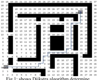
tentative distance dist(v). If the one via v is shorter, we update dist(v) and v in the priority queue. The algorithm terminates once the priority queue is empty; this happens after at most n steps, where n is the number of nodes in the graph. After the termination, all nodes are either unreached or settled. Shortest-path tree can be determined with the help of the parent-pointer. Fig. 1 shows an example Dijkstra’s algorithm in a grid environment of 20 by 20. Each grid cell has a value of the smallest distance between its self and source. The source is located at cell (2, 3) and target is located at cell (18, 18) while there are static obstacles within the environment that occupied some cells as can be seen from the figure.

Fig 1: shows Dijkstra algorithm determine shortest path in grid environment.

To address the issue of SSSP, Dijkstra algorithm operates by finding the next node to move with least cost of traversing. If there are two nodes with same cost, it arbitrary chooses any one of those nodes and move on. For example, looking at the figure above, at the source location there are two nodes with the same cost that will lead to the shortest-path to reach the target; Dijkstra will randomly choose one move to the next node.

The following is an algorithm that shows how Dijkstra operate:

STEP 1: Choose the source cell from

the set Q of free cells

STEP 2: Create an empty set R to store

those cells to which the shortest path has been found.

STEP 3: Initialize the chosen source

cell s with distance of travelling d(s) = 0 and parent pointer p(s) = s and add it to R. For all other cells v in Q d(v) = infinity and p(v) = null.

STEP 4: For all cell V in Q that is

among the four neighboring cell of v, d(v) = d(u) + 1.

But if v was assign a distance d(v) via other neighboring cells of v, then the new distance will be min( distance of the recently added cell to S + 1, old distance of v). Assign a parent pointer to cell v: p(v) = u

STEP 5: Pick a cell u in Q with the

smallest distance and it to R if there are more one cell with smallest distance, choose arbitrary.

STEP 6: Repeat step 5 until the target

cell is in R or until all the cells are in R. To get the shortest path;

STEP 7: Create an empty set S

STEP 8: Let the target cell be v

STEP 9: Add v to the set S

STEP 10: Let the parent pointer of v be u

(note that v may be chosen arbitrary since cell with the same distance are chosen arbitrary)

STEP 11: If u is the same as v, add u to S

STEP 12: Repeat 5 until u is the same as

v.

4. ENVIRONMENTAL MODELING AND

PATH PLANNING

361 square grids. Each shall either be free or occupied and shall appropriately contained the obstacles or be free at all to avoid a collision. From the free cells, those that contained doorways, junctions, curves, corners and free positions inside a room are identified, located and marks as critical grids. Two critical cells are considered adjacent if there are free cells to allow feasible passage between them. These are then interconnected to form the multiple possible paths from which the user can choose.

The interconnection of these critical cells formed a network graph. Dijkstra shortest path algorithm shall be used to find the shortest path between any two of these critical cells with the cells as the vertices and distances as the edges. The distances are calculated using the locations of the vertices in the two-dimensional space computed by the RFID. Assuming we want find a distance

between two points on the search space say cell1

and cell2. The distance between these points can

be computed using the following equation:

Distance = | celly,2 – celly,1 | + | cellx,2 – cell |

Where celly,2 means value of cell2 in y-axis.

The following is the algorithm of the proposed model:

STEP 1: Choose the source cell from

the set Q of free cells

STEP 2: Create an empty set R to store

those cells to which the shortest path has been found.

STEP 3: Initialize the chosen source

cell s with distance of

travelling d(s) = 0, a status s(s) = permanent and parent pointer p(s) = s and add it to R. For all other cells v in Q d(v) = infinity, s(v) = temporary and p(v) = null.

STEP 4: Locate all the critical cells in

Q. Consider each critical cell v in Q that can be reach directly from the recently added cell u to R. compute distance of travelling between u and v (i.e. d(u, v)) and assign v a distance d(v) = d(u) + d(u, v). But if v was assign a distance d(v) via other critical cells that can be reach directly from v (

by our computation), then, new distance of v is:

min(d(u) + d(u, v), old distance of v) of v

p(v) = u s(u) = visited

STEP 5: Pick a cell u in Q with the

status s(u) = visited that has smallest distance and it to R. Now p(u) = permanent

STEP 6: Repeat step 5 until the target

cell is in R or until no any visited cell is in R.

To get the shortest path;

STEP 7: Create an empty set S

STEP 8: Let the target cell be v

STEP 9: Add v to the set S

STEP 10: Compute the number of the junction of each and every parent cell.

STEP 11: Choose among the parent of v

a parent with a minimum number of junctions and add it to S.

STEP 12: Repeat step 5 until u is the

same as v.

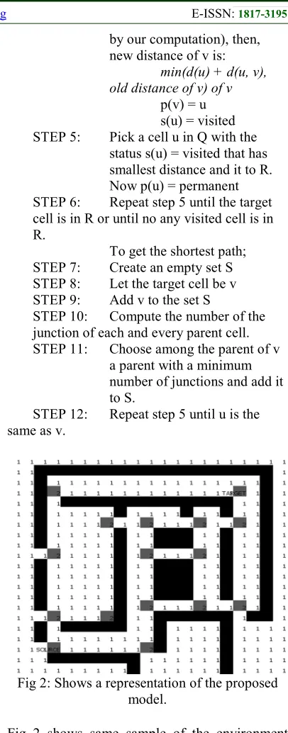
Fig 2: Shows a representation of the proposed model.

362

5. SIMULATION AND RESULTS

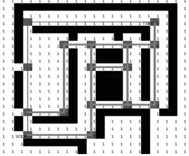
Three (3) predefined maps of the terrain have been developed in a grid environments to simulate the shortest path calculations. They represent three different size of grids; (i) 15 by 15, (ii) 20 by 20 and (iii) 25 by 25 grids. Figure 1 shows the 20 by 20 map with its shortest path calculated by the traditional Dijkstra’s algorithm while Fig. 3 shows its possible paths with thick lines and the selected shortest path with a thin line for the map calculated by the proposed algorithm.

Fig. 3 show shortest path generated and movement of the robot within the simulated

environment

The shortest path is selected based on the number of junctions. This is to minimize use of path with T-junction due the possibility of collision with other robots that are within the terrain. This can be deduced from the above figure. There are six feasible paths of which three have five T-junctions; the remaining three has four, three and one T-junctions. The robot decides to choose path with one T-junction and move along it. The cell with the label “Source” indicates the starting point while cell with the label “Target” indicates the destination point.

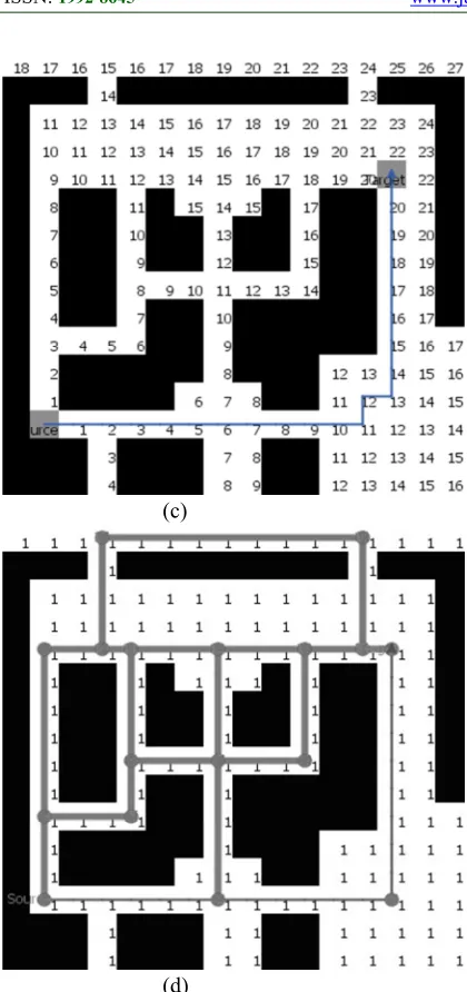
Fig. 4(a) shows a simulation result of 25 by 25 using traditional Dijkstra while Fig 4(b) shows the result of the proposed model. Whereas, Fig. 4(c) shows a simulation result of 15 by 15 using traditional Dijkstra and Fig 4(d) shows the result of the proposed model. The thick line in Fig. 4(b) and 4(d) indicates feasible paths identified while the thin line with the directed arrow indicates the shortest path chosen by the proposed algorithm to move from the source point to the destination. The starting point and

destination of the robot is the same for both traditional Dijkstra and our proposed model.

(a)

(b)

363

(c)

(d)

The simulation results show that the proposed algorithm performs better in every aspect in every map. The proposed algorithm only considers the critical cells in its path; therefore it

reduces the possible number of cells

significantly, hence the number of possible paths identified and the calculation time taken. Regardless of the small number of possible paths identified and the shorter calculation time, the proposed algorithm managed to identify the shortest path with the same length or distance with the traditional algorithm. In the traditional algorithm, whenever more than one path with minimum length is found, the shortest path will be selected arbitrarily, whereas the proposed algorithm will choose the path with the

minimum number of junctions. Therefore the shortest path identified by the proposed algorithm is the most optimal path.

Table 1: Results Comparison Between The Traditional Dijkstra And The Proposed Algorithm

Dijks tra

15 by 15 grids

20 by 20 grids

25 by 25 grids

Tra ditio

nal Pro pos ed

Tra ditio nal

Pro pos ed

Tra ditio

nal Pro pos ed Possi

ble cells

225 17 400 13 625 16

Possi ble path ident ified

14 7 33 6 28 4

Calc ulati on time/ s

0.03 0.0

2

0.05 0.0

3

0.09 0.0

2

Chos en path

Ran dom

Mo st opt im al

Ran dom

Mo st opt im al

Ran dom

Mo st opt im al Leng

th (/unit )

21 21 31 31 32 32

6. CONCLUSION

364

Acknowledgment: This research is supported by the Kano State Government Nigeria and Universiti Sultan Zainal Abidin.

REFERENCES:

[1] Kala, R., Shukla, A., & Tiwari, R. (2009,

November). Robotic path planning using

multi neuron heuristic search.

In Proceedings of the 2nd International

Conference on Interaction Sciences:

Information Technology, Culture and

Human (pp. 1318-1323). ACM.

[2] Dijkstra, E. W. (1959). A note on two

problems in connexion with

graphs.Numerische mathematik, 1(1), 269-271.

[3] Mansouri, M., Shoorehdeli, M. A., & Teshnehlab, M. (2008, October). Path planning of mobile robot using integer ga

with considering terrain conditions.

InSystems, Man and Cybernetics, 2008.

SMC 2008. IEEE International Conference on (pp. 208-213). IEEE.

[4] Ismail, A. T., Sheta, A., & Al-Weshah, M. (2008). A mobile robot path planning using

genetic algorithm in static

environment. Journal of Computer

Science,4(4), 341.

[5] Soofiyani, F. R., Rahmani, A. M., & Mohsenzadeh, M. (2010, July). A Straight Moving Path Planner for Mobile Robots in

Static Environments Using Cellular

Automata. In Computational Intelligence,

Communication Systems and Networks

(CICSyN), 2010 Second International

Conference on (pp. 67-71). IEEE.

[6] Ying-hua, X., & Hong-peng, L. (2010, May). Optimal Path Planning for Service Robot in Indoor Environment. In Intelligent Computation Technology and Automation (ICICTA), 2010 International Conference on (Vol. 2, pp. 850-853). IEEE.

[7] Ahmed, S. U., Malik, U. A., Iqbal, K. F., Ayaz, Y., & Kunwar, F. (2011, August). Sparsed potential-PCNN for real time path planning and indoor navigation scheme for

mobile robots. In Mechatronics and

Automation (ICMA), 2011 International

Conference on (pp. 1729-1734). IEEE.

[8] Jin, X. B. (2013, August). Fusion Estimation Based on UKF for Indoor RFID Tracking.

In Green Computing and Communications

(GreenCom), 2013 IEEE and Internet of

Things (iThings/CPSCom), IEEE

International Conference on and IEEE Cyber, Physical and Social Computing (pp. 1928-1931). IEEE.

[9] Reza, A. W., Geok, T. K., & Dimyati, K. (2011). Tracking via square grid of RFID

reader positioning and diffusion

algorithm. Wireless Personal

Communications, 61(1), 227-250.

[10]Hongling, H., & Fenglei, Y. (2010, November). Path Planning of an Indoor Mobile Robot Navigated by Infrared. In E-Product E-Service and E-Entertainment (ICEEE), 2010 International Conference on (pp. 1-4). IEEE. Hongling, H., & Fenglei, Y. (2010, November). Path Planning of an Indoor Mobile Robot Navigated by Infrared.

In E-Product E-Service and