Simulation and Evaluation of Shrinkage Techniques for Image De-noising under Additive White Gaussian Noise (AWGN)

(1)

Simulation and Evaluation of Shrinkage Techniques for

Image De-noising under Additive White Gaussian Noise

(AWGN)

Virendra Kumar, Dr. Ajay Kumar

Electronics and Communication Engineering, BCET, Gurdaspur, Punjab, India

,

Abstract- Image denoising is a process to restore a worth

image from degraded image by choosing an appropriate filter but choosing an appropriate filter still is a challenge. Recently, wavelet transform has attracted more and more interest in image de-noising because the wavelet transform of an image produces a non-redundant image representation, which provides better spatial and spectral localization of image formation. The wavelet transform can be interpreted as image decomposition in a set of independent, spatially oriented frequency channels and each cannel can be treated as a single element for removal of noise using an appropriate shrinkage threshold and at the end all treated channels recombined to get denoised image. We discuss in this paper various shrinkage techniques used in wavelet transform for image denoising in respect of test image size, orthogonal wavelets and elapsed time under Additive White Gaussian Noise.

Index Terms- Additive White Gaussian Noise (AWGN), Image Denoising, Peak Signal to Noise Ratio (PSNR), Shrinkage Techniques, and Wavelet Transform.

I. INTRODUCTION

he image denoising [1, 2] of an image naturally corrupted by noise is a classical problem in the field of image processing. In image processing, noise is undesired information that degrades the quality of image. Imperfect instruments, problems with the data acquisition process, and interfering natural phenomena can degrade the data of interest. Image denoising involves removing the effect of noise and preserves the detail to produce a high quality image. There are various methods to restore an image from noisy distortions but selecting the appropriate method plays a major role in getting the desired image. The denoising methods tend to be problem specific. For example, a method that is used to denoise satellite images may not be suitable for denoising medical images. This paper covers the wavelet transform shrinkage techniques for image denoising and their detail comparative study. The performance of each technique is compared by computing Mean Square Error (MSE) and Peak Signal to Noise Ratio (PSNR) [3, 4] besides the visual interpretation.

II. WAVELET TRANSFORM SHRINKAGE TECHNIQUES

Donoho and Johnstone [5] pioneered the work on filtering of additive Gaussian noise using wavelet thresholding. From their properties and behavior, wavelets play a major role in image

denoising. The term wavelet thresholding is explained as decomposition of the image into wavelet coefficients, comparing the detail coefficients with a given threshold value, and shrinking these coefficients close to zero to take away the effect of noise in the image. The image is reconstructed from the modified coefficients. This process is also known as the inverse discrete wavelet transform. During thresholding, a wavelet coefficient is compared with a given threshold and is set to zero if its magnitude is less than the threshold; otherwise, it is retained or modified depending on the threshold rule.

Thresholding methods use a threshold and determine the clean wavelet coefficients based on this threshold.

A. Hard Thresholding

If the absolute value of a coefficient is less than a threshold, then it is assumed to be 0, otherwise it is unchanged. Mathematically it is given by

fh(x) = x, if x ≥ λ

= 0, otherwise

The hard thresholding [6] function chooses all wavelet coefficients that are greater than the given threshold λ and sets the others to zero. The threshold λ is chosen according to the signal energy and the noise variance (σ 2_).

B. Soft Thresholding

The soft thresholding [6] function has a somewhat different rule from the hard thresholding function. It shrinks the wavelet coefficients by λ towards zero,

Hard thresholding is discontinuous. To overcome this, Donoho introduced the Soft Thresholding method. If the absolute value of a coefficient is less than the threshold λ, then it is assumed to be 0, otherwise its value is shrunk by λ. Mathematically, it is given by

f (x) = x ‒ λ, if x ≥ λ = 0, if x < λ = x + λ, if x λ

The soft-thresholding rule is chosen over hard-thresholding, because soft-thresholding method yields more visually pleasant images over hard thresholding.

C. Visu Shrink

Visu Shrink [6] was introduced by Donoho. It uses a threshold value T that is proportional to the standard deviation of the noise. It follows the hard thresholding rule. It is also referred to as universal threshold and is defined as

(2)

(1)

where σ 2 is the noise variance and M is the number of pixels. This asymptotically yields a MSE estimate as M tends to infinity. As M increases, we get bigger and bigger threshold, which tends to over smoothen the image. Visu Shrink follows the global thresholding [6] scheme where there is a single value of threshold applied globally to all the wavelet coefficients [1].

D. Bayes Shrink

Bayes Shrink [7] was proposed by Chang, Yu and Vetterli [8]. It uses soft thresholding and is subband dependent, which means that thresholding is done at each band of resolution in the wavelet decomposition. It is smoothness adaptive. In particular, it is assumed that, for the various subbands and decomposition levels, the wavelet coefficients of the original image follow approximately a Generalized Gaussian Distribution (GGD) [4]. The Bayes threshold ‘T’ is defined as

(2)

if is non-zero.

Otherwise, it is set to some predetermined maximum value.

(3) is calculated as,

(4)

The noise variance is estimated from the HH band as,

(5)

D. Neigh Shrink

In NeighShrink [9] method, the wavelet coefficients are threshold according to the magnitude of the squared sum of all the wavelet coefficients i.e. the local energy within the neighborhood window.

Let d(i,j) denote the wavelet coefficients of interest and B(i,j) is a neighborhood window around d(i,j). Also let S2=Σd2(i,j) over the window B(i,j). Then the wavelet coefficient to be threshold, is shrinked according to the formulae,

d(i,j)= d(i,j)* B(i,j) (6) where the shrinkage factor can be defined as B(i,j) = ( 1-T2/ S2(i,j))+, and the sign + at the end of the formulae means to keep

the positive value while set it to zero when it is negative.

E. Gaussian Noise

Gaussian noise is evenly distributed over the signal [10]. This means that eachpixel in the noisy image is the sum of the true pixel value and a random Gaussiandistributed noise value. As the name indicates, this type of noise has a Gaussiandistribution, which has a bell shaped probability distribution function given by,

(7) where g represents the gray level, m is the mean or average of the function, and σ is the standard deviation of the noise.

g

Fig.1Gaussian distribution

III. PERFORMANCE MEASURE

To measure the performance of the various shrinkage techniques for image denoising, a test image is added with some known Gaussian noise. This would then be given as input to the denoising algorithm, which produces an image close to the original test image as per shrinkage techniques deployed. The performance of each shrinkage algorithm is compared by computing MSE and PSNR, besides the visual interpretation.

MSE and PSNR are the two main parameters for comparison of shrinkage denoising techniques. In statistics, the mean squared error of an estimator is the difference between an estimator and the true value of the quantity being estimated i.e. difference between the original image and the denoised image.

Let original image is of size and is

estimated image after restoration then MSE can be defined as-

(8) PSNR is the peak signal to noise ratio, here signal is the original image and noise is error introduced by restoration. PSNR is the most commonly used parameter to measure the quality of reconstruction image with respect to the original image. A higher PSNR would normally indicate that the reconstruction is of higher quality. PSNR is usually expressed in terms of the logarithmic decibel scale (dB).

(9) Using (8), we get

(10)

Here is the original image of size and is

the reconstructed image after restoration. In the expression of

(3)

PSNR, the value of the numerator is 2552; it is the square of the maximum possible pixel value of the image . When is the 8-bit gray scale image, the maximum possible pixel value of the Image is 255.

Elapsed Time is the amount of time which MATLAB takes to complete all operations of that particular denoising algorithms and displays the time in seconds.

IV. SIMULATED RESULTS AND DISCUSSION

The wavelet transforms shrinkage methods: Visu Shrink, Bayes Shrink, Neigh Shrink, Bi Shrink are simulated in MATLAB. The test images: Lena, Barbara and Boats of sizes 512×512 and House and Peppers of sizes 256×256 are corrupted with AWGN of standard deviation sigma at different intervals i.e. sigma (σ) = 10, 20, 30, 40.The wavelets used are orthogonal wavelets i.e. coiflets, symlets, daubechies and haar.

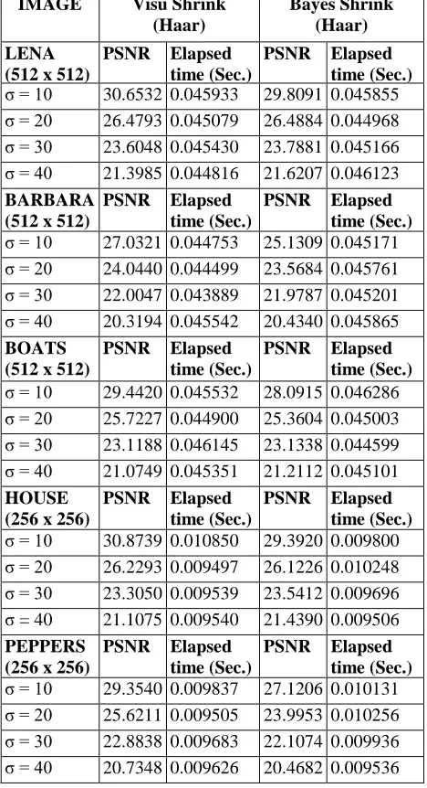
Table-1(a) Performance under different sigma values of AWGN

IMAGE Visu Shrink (Haar)

Bayes Shrink (Haar)

LENA (512 x 512)

PSNR Elapsed time (Sec.)

σ = 10 30.6532 0.045933 29.8091 0.045855 σ = 20 26.4793 0.045079 26.4884 0.044968 σ = 30 23.6048 0.045430 23.7881 0.045166 σ = 40 21.3985 0.044816 21.6207 0.046123

BARBARA (512 x 512)

σ = 10 27.0321 0.044753 25.1309 0.045171 σ = 20 24.0440 0.044499 23.5684 0.045761 σ = 30 22.0047 0.043889 21.9787 0.045201 σ = 40 20.3194 0.045542 20.4340 0.045865

BOATS (512 x 512)

σ = 10 29.4420 0.045532 28.0915 0.046286 σ = 20 25.7227 0.044900 25.3604 0.045003 σ = 30 23.1188 0.046145 23.1338 0.044599 σ = 40 21.0749 0.045351 21.2112 0.045101

HOUSE (256 x 256)

σ = 10 30.8739 0.010850 29.3920 0.009800 σ = 20 26.2293 0.009497 26.1226 0.010248 σ = 30 23.3050 0.009539 23.5412 0.009696 σ = 40 21.1075 0.009540 21.4390 0.009506

PEPPERS (256 x 256)

σ = 10 29.3540 0.009837 27.1206 0.010131 σ = 20 25.6211 0.009505 23.9953 0.010256 σ = 30 22.8838 0.009683 22.1074 0.009936 σ = 40 20.7348 0.009626 20.4682 0.009536

Table-1(b) Performance under different sigma values of AWGN

IMAGE Neigh Shrink

(Haar)

Bi Shrink (Haar)

LENA (512 x 512)

PSNR Elapsed time (Sec.)

σ = 10 33.3147 5.800438 32.7335 0.047611

σ = 20 29.7907 5.676601 29.0275 0.047452

σ = 30 27.9265 5.704856 26.8363 0.061307

σ = 40 26.6950 5.607180 25.2176 0.045770

BARBARA (512 x 512)

σ = 10 31.5857 5.922542 30.3805 0.048614

σ = 20 27.4689 5.792790 26.0484 0.047630

σ = 30 25.3808 5.723764 24.0034 0.047934

σ = 40 24.0829 5.702113 22.6938 0.048180

BOATS (512 x 512)

σ = 10 31.9014 5.855568 31.3918 0.048494

σ = 20 28.2986 5.706110 27.7366 0.047814

σ = 30 26.4013 5.687567 25.6460 0.045968

σ = 40 25.2007 5.663731 24.1534 0.045849

HOUSE (256 x 256)

σ = 10 33.5719 1.486125 33.0123 0.010874

σ = 20 29.9426 1.444289 29.1771 0.011689

σ = 30 27.9873 1.476113 26.7781 0.010377

σ = 40 26.6621 1.419338 24.9968 0.011341

PEPPERS (256 x 256)

σ = 10 32.0660 1.488034 31.3745 0.011141

σ = 20 27.9119 1.461632 27.5441 0.011296

σ = 30 25.7133 1.426746 25.2915 0.011394

σ = 40 24.1687 1.418810 23.6835 0.011752

The all wavelet transform shrinkage methods are applied on all five test images with the combination of four wavelets coif5, sym8, db10 and harr for image denoising using Gaussion noise sigma variation from 10 to 40. The simulated results with haar wavelet are tabulated as given above Table - 1(a) and 1(b) and the following graphs (in Fig 2 to Fig 5) represent the comparative views of each shrinkage method with four wavelets coif5, sym8, db10 and harr applied to all test images i.e. Lena, Barbara and Boats of sizes 512×512 and House and Peppers of sizes 256×256.

[image:3.612.327.564.94.527.2] [image:3.612.51.285.298.729.2]

(4)

10 15 20 25 30 35 40 20

22 24 26 28 30 32 34 35

SIGMA

P

S

N

R

(

db

)

NEIGH SHRINK (coif5)

LENA (512 x 512) BARBARA (512 x 512) BOATS (512 x 512) HOUSE (256 x 256) PEPPERS (256 x 256)

Fig.2(a) Performance Neigh Shrink using coif5 wavelet

10 15 20 25 30 35 40

20 22 24 26 28 30 32 34 35

BAYES SHRINK (coif5)

SIGMA

P

S

N

R

(

d

b

)

Fig.2(b) Performance Bayes Shrink using coif5 wavelet

10 15 20 25 30 35 40

20 22 24 26 28 30 32 34 35

VISU SHRINK (coif5)

SIGMA

P

S

N

R

(

d

b

)

LENA (512x512) BARBARA (512x512) BOATS (512x512) HOUSE (256 x 256) PEPPERS (256 x 256)

Fig.2(c) Performance Visu Shrink using coif5 wavelet

10 15 20 25 30 35 40

20 22 24 26 28 30 32 34 35

NEIGH SHRINK (sym 8)

SIGMA

P

S

N

R

(

db

)

Fig.3(a) Performance Neigh Shrink using sym8 wavelet

10 15 20 25 30 35 40

20 22 24 26 28 30 32 34 35

BAYES SHRINK (sym 8)

SIGMA

P

S

N

R

(

d

b

)

LENA (512 x 512) BARBARA (512 x 512) BOATS (512 x 512) HOUSE (256 x 256) HOUSE (256 x 256)

Fig.3(b) Performance Bayes Shrink using sym8 wavelet

10 15 20 25 30 35 40

20 22 24 26 28 30 32 34 35

VISU SHRINK (sym 8)

SIGMA

P

S

N

R

(

d

b

)

(5)

10 15 20 25 30 35 40 20

22 24 26 28 30 32 34 35

NEIGH SHRINK (db10)

SIGMA

P

S

N

R

(

d

b

)

Fig.4(a) Performance Neigh Shrink using db10 wavelet

10 15 20 25 30 35 40

20 22 24 26 28 30 32 34 35

BAYES SHRINK (db10)

SIGMA

P

S

N

R

(

d

b

)

LENA (512 x 512) BARBARA (512 x 512) BOATS (512 x 512) HOUSE (256 x256) PEPPERS (256 x256)

Fig.4(b) Performance Bayes Shrink using db10 wavelet

10 15 20 25 30 35 40

20 22 24 26 28 30 32 34 35

VISU SHRINK (db10)

SIGMA

P

S

N

R

(

db

)

Fig.4(c) Performance Visu Shrink using db10 wavelet

10 15 20 25 30 35 40

20 22 24 26 28 30 32 34 35

NEIGH SHRINK (Haar)

SIGMA

P

S

N

R

(

d

b

)

Fig.5(a) Performance Neigh Shrink using haar wavelet

10 15 20 25 30 35 40

20 22 24 26 28 30 32 34 35

BAYES SHRINK (Haar)

SIGMA

P

S

N

R

(

d

b

)

Fig.5(b) Performance Bayes Shrink using haar wavelet

10 15 20 25 30 35 40

20 22 24 26 28 30 32 34 35

VISU SHRINK (Haar)

SIGMA

P

S

N

R

(

d

b

)

(6)

ORIGNAL IMAGE

Fig.6(a) Original Test Image LENA (512 x 512)

NOISY IMAGE (GAUSSION SIGMA = 30)

Fig.6(b) Noisy Image with Gaussion Noise (σ = 30)

DENOISED IMAGE AT GAUSSION NOISE SIGMA = 30)

Fig.6(c) Denoised Image with Neigh Shrink method using coif5 wavelet at Gaussion Noise (σ = 30)

V. CONCLUSION

The PSNR and elapsed time (execution time) are taken as performance measures. The PSNR values and elapsed time of the different filters for various test images are tabulated in table 1 and different shrinkage techniques for orthogonal wavelets are graphed in Fig 2 to Fig 5.These simulated result shows that the Neigh Shrink method with coif5 wavelet gives best performance (high PSNR) at the cost of more execution time (elapsed time) among all used shrinkage methods for image denoising in respect of different test images and their size. The performance of wavelets coif5 and sym8, haar and db1 are almost same in terms of PSNR values. The filter with less elapsed time is usually implemented in real-time applications.

REFERENCES

[1] R. C. Gonzalez and R. E. Woods, Digital Image Processing, Prentice-Hall, India, second edition, 2007.

[2] A.K.Jain,Fundamentals of digital Image processing. Prentice-Hall, 1989. [3] R. Yang, L. Yin, M. Gabbouj, J. Astola, and Y. Neuvo, “Optimal weighted

median filters under structural constraints,”IEEE Trans. Signal Processing,vol.43, pp.591–604, Mar.1995.

[4] Martin Vetterli S Grace Chang, Bin Yu, “Adaptive Wavelet Thresholding for Image and Compression,” IEEE Transactions on Image Processing,

9(9):1532–1546, Sep 2000.

[5] David L. Donoho and Iain M. Johnstone, “Adapting to UnknownSmoothness via Wavelet Shrinkage,” Journal of American StatisticalAssociation, 90(432):1200-1224, Dec 1995.

[6] D. L. Donoho, “De-noising by soft-thresholding”,IEEE Trans. Information Theory, vol.41, no.3, pp.613-627, May1995.

[7] E. P. Simoncelli and E. H. Adelson. Noise removal via Bayesian wavelet coring. In Third Int'l Conf on Image Proc, volume I, pages 379-382, Lausanne, September 1996. IEEE Signal Proc Society.

[8] S. G. Chang, B. Yu and M. Vetterli, Adaptive wavelet thresholding for Image Denoising and compression, IEEE Trans. on Image Proc., vol. 9, no. 9, pp. 1532-1546, Sept. 2000.

[9] Dr. S. Arumuga Perumal, Dr. M.Mohamed Sathik, S.Kother Mohideen, “Image Denoising Using Discrete Wavelet Transform”International Journal of Computer Science and Network Security (IJCSNS), Volume 8, Issue 1, pp. 213-216, January 2008.

[10] Scott E Umbaugh, Computer Vision and Image Processing, Prentice Hall PTR, New Jersey, 1998.

AUTHORS

Er. Virendra Kumar, pursuing M. Tech., Department of Electronics & Communication Engineering, Beant College of Engineering & Technology, Gurdaspur, Punjab, Email: [email protected].

Dr. Ajay Kumar, Associate Professor, Department of Electronics and Communication Engineering, Beant College of Engineering & Technology, Gurdaspur, Punjab, Email: [email protected].

Correspondence Author – Virendra Kumar, Email:

[email protected], contact number –