Study of Efficient technique based on Entropic
Threshold for edge detection in Bone Marrow Images
Sathish K R*, Swaroop M*, Achudan TS**, Vishnupriya R ***
* B.E, Electronics and Instrumentation Engineering, St. Joseph’s College of Engineering, Chennai, India * *B.E, Electrical and Electronics Engineering, Mepco Schlenk Engineering College, Sivakasi, India *** M.Tech, Electronics and Instrumentation Engineering, St. Joseph’s College of Engineering, Chennai, India
DOI: 10.29322/IJSRP.9.12.2019.p9688
http://dx.doi.org/10.29322/IJSRP.9.12.2019.p9688
Abstract- Thresholding is an important task in image processing. It is a main tool in pattern recognition, image segmentation, edge detection and scene analysis. In this paper, we present a new thresholding technique based on Tsallis and shannon entropy. The main advantages of the proposed method are its robustness and its flexibility. We present experimental results for this method, and compare results of the algorithm against several leading-edge detection methods, such as Canny and Sobel. Experimental results demonstrate that the proposed method achieves better result than some classic methods and the quality of the edge detector of the output images is robust.
Index Terms- Entropy Threshold, Edge Detection, Shannon and Tsallis Entropy
I.
INTRODUCTIONImage Segmentation
Image segmentation procedure is used to extract the key features from the unprocessed input image. Thresholding is a reputed image segmentation technique used to obtain binary image from the gray level image. In the literature, a considerable number of Thresholding procedures are available to segment the Gray scale and RGB images.
In imaging science, image processing plays a vital role in the analysis and interpretation of images in fields such as medical discipline, navigation, environment modeling, automatic event detection, surveillance, texture and pattern recognition, and damage detection. The development of digital imaging techniques and computing technology increased the potential of imaging science.
Image segmentation is one of pre-processing techniques used to regulate the features of an image. Image segmentation is judged as an important procedure for significant examination and interpretation of input images.
In segmentation, the input image is separated into non-overlapping, homogenous regions containing similar objects. Based on the performance appraisal process, the segmentation methods are classified into two groups such as supervised and unsupervised evaluation. Unsupervised methods are preferable in real-time processing because they do not require a manually segmented image.
Thresholding
Thresholding is considered the most desired procedure out of all the existing procedures used for image segmentation, because of its simplicity, robustness, accuracy and competence. If the input image is divided into two classes, such as the background and the object of interest, and is called bi-level Thresholding. Bi-level Thresholding is extended to multi-level Thresholding to obtain more than two classes.
The thresholds can be derived at a local or global level. In local thresholding, a different threshold is assigned for each part of the image, while in global thresholding, a single global threshold the probability density function of the grey level histogram can be handled by a parametric or a nonparametric approach to find the thresholds. In the parametric approaches, the statistical parameters of the classes in the image are estimated. They are computationally expensive, and their performance may vary depending on the initial conditions. In the nonparametric approaches, the thresholds are determined by maximizing some criteria, such as between-class variance or entropy measures. In information theory, entropy is the measurement of the indeterminacy in a random variable[5]. The methods such as Kapur, Shannon, Tsallis, and Otsu are widely adopted by most of the researchers to find solution for multilevel image segmentation problems . In general, Kapur and Otsu based thresholding techniques proved for their better shape and uniformity measures for the bi-level and multi-level thresholding problems.
Recent literature illustrates that a number of heuristic and meta-heuristic algorithms are employed to segment the gray scale and RGB images.
Edge detection
Edge detection includes a variety of mathematical methods that aim at identifying points in a digital image at which the image brightness changes sharply or, more formally, has discontinuities. The points at which image brightness changes sharply are typically organized into a set of curved line segments termed edges. The same problem of finding discontinuities in one-dimensional signals is known as step detection and the problem of finding signal discontinuities over time is known as change detection. Edge detection is a fundamental tool in image processing, machine vision and computer vision, particularly in the areas of feature detection and feature extraction.
Methodology
Image processing is a general term for the wide range of techniques that are used to manipulate, modify or classify images in various ways. In general, a digital image acquired through digital camera is used for analysis through computers. In the literature, a number of image thresholding procedures are available for gray scale and RGB image segmentation procedures.
The other edge detection procedures such as canny, sobel, and robert are very efficient and successful in the case of bi-level thresholding process. When the number of threshold level increases, classical thresholding techniques produces low quality images.
Sobel Algorithm Method
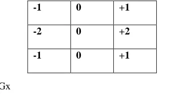
The operator consists of a pair of 3×3 convolution kernels as shown in Figure 3.1. One kernel is simply the other rotated by 90°[2].
Gx Gy
Figure 1.1: Masks used by Sobel Operator
These kernels are designed to respond maximally to edges running vertically and horizontally relative to the pixel grid, one kernel for each of the two perpendicular orientations. The kernels can be applied separately to the input image, to produce separate measurements of the gradient component in each orientation (call these Gx and Gy). These can then be combined together to find the absolute magnitude of the gradient at each point and the orientation of that gradient[3]. The gradient magnitude is given by:
|G| = √ ( Gx2 + Gy2 ) (1.1)
Typically, an approximate magnitude is computed using:
|G| = |Gx| + |Gy| (1.2) which is much faster to compute.
The angle of orientation of the edge (relative to the pixel grid) giving rise to the spatial gradient is given by:
θ = arctan (Gy / Gx). (1.3)
Robert’s cross operator:
The Roberts Cross operator performs a simple, quick to compute, 2-D spatial gradient measurement on an image[10]. Pixel values at each point in the output represent the estimated absolute magnitude of the spatial gradient of the input image at that point. The operator consists of a pair of 2×2 convolution kernels as shown in Figure 3.2. One kernel is simply the other rotated by 90°. This is very similar to the Sobel operator.
-1 0 +1
-2 0 +2
-1 0 +1
+1 0 +1
0 0 0
Gx Gy
Figure 1.2 : Masks used for Robert operator.
These kernels are designed to respond maximally to edges running at 45° to the pixel grid, one kernel for each of the two perpendicular orientations. The kernels can be applied separately to the input image, to produce separate measurements of the gradient component in each orientation (call these Gx and Gy). These can then be combined together to find the absolute magnitude of the gradient at each point and the orientation of that gradient. The gradient magnitude is given by:
|G| = √(Gx2 + Gy2) (1.4)
Although typically, an approximate magnitude is computed using:
|G|=|Gx| + |Gy| which is much faster to compute.
The angle of orientation of the edge giving rise to the spatial gradient (relative to the pixel grid orientation) is given by:
θ = arctan (Gy /Gx) − 3π/ 4. (1.5)
Canny Edge Detection Algorithm:
The Canny edge detection algorithm is known to many as the optimal edge detector. The first and most obvious is low error rate. It is important that edges occurring in images should not be missed and that there be no responses to non-edges. The second criterion is that the edge points be well localized. In other words, the distance between the edge pixels as found by the detector and the actual edge is to be at a minimum. A third criterion is to have only one response to a single edge. This was implemented because the first two were not substantial enough to completely eliminate the possibility of multiple responses to an edge. Based on these criteria, the canny edge detector first smoothes the image to eliminate and noise. It then finds the image gradient to highlight regions with high spatial derivatives. The algorithm then tracks along these regions and suppresses any pixel that is not at the maximum (no maximum suppression). The gradient array is now further reduced by hysteresis. Hysteresis is used to track along the remaining pixels that have not been suppressed[4]. Hysteresis uses two thresholds and if the magnitude is below the first threshold, it is set to zero (made a non edge). If the magnitude is above the high threshold, it is made an edge. And if the magnitude is between the 2 thresholds, then it is set to zero unless there is a path from this pixel to a pixel with a gradient above T2.
Step 1: In order to implement the canny edge detector algorithm, a series of steps must be followed. The first step is to filter out any noise in the original image before trying to locate and detect any edges. And because the Gaussian filter can be computed using a simple mask, it is used exclusively in the Canny algorithm. Once a suitable mask has been calculated, the Gaussian smoothing can be performed using standard convolution methods. A convolution mask is usually much smaller than the actual image. As a result, the mask is slid over the image, manipulating a square of pixels at a time. The larger the width of the Gaussian mask, the lower is the detector's sensitivity to noise. The localization error in the detected edges also increases slightly as the Gaussian width is increased.
Step 2: After smoothing the image and eliminating the noise, the next step is to find the edge strength by taking the gradient of the image. The Sobel operator performs a 2-D spatial gradient measurement on an image. Then, the approximate absolute gradient magnitude (edge strength) at each point can be found. The Sobel operator uses a pair of 3x3 convolution masks, one estimating the gradient in the x-direction (columns) and the other estimating the gradient in the y-direction (rows).
Gx Gy
Figure 1.3: Masks used for canny operator.
+1 0
0 -1
0 +1
-1 0
-1 0 +1
-2 0 +2
-1 0 +1
+1 +2 +1
0 0 0
The magnitude, or edge strength, of the gradient is then approximated using the formula:
|G| = |Gx| + |Gy|. (1.6)
Step 3: The direction of the edge is computed using the gradient in the x and y directions. However, an error will be generated when sum is equal to zero. So in the code there has to be a restriction set whenever this takes place. Whenever the gradient in the x direction is equal to zero, the edge direction has to be equal to 90 degrees or 0 degrees, depending on what the value of the gradient in the y-direction is equal to. If GY has a value of zero, the edge y-direction will equal 0 degrees. Otherwise the edge y-direction will equal 90 degrees. The formula for finding the edge direction is just:
θ = tan-1 (Gy / Gx). (1.7)
Step 4: Once the edge direction is known, the next step is to relate the edge direction to a direction that can be traced in an image. So if the pixels of a 5x5 image are aligned as follows:
X x x x x
X x x x x
X x x x x
X x x x x
X x x x x
Then, it can be seen by looking at pixel "a", there are only four possible directions when describing the surrounding pixels - 0 degrees (in the horizontal direction), 45 degrees (along the positive diagonal), 90 degrees (in the vertical direction), or 135 degrees (along the negative diagonal). So now the edge orientation has to be resolved into one of these four directions depending on which direction it is closest to (e.g. if the orientation angle is found to be 3 degrees, make it zero degrees). Think of this as taking a semicircle and dividing it into 5 regions. Therefore, any edge direction falling within the yellow range (0 to 22.5 & 157.5 to 180 degrees) is set to 0 degrees. Any edge direction falling in the green range (22.5 to 67.5 degrees) is set to 45 degrees. Any edge direction falling in the blue range (67.5 to 112.5 degrees) is set to 90 degrees. And finally, any edge direction falling within the red range (112.5 to 157.5 degrees) is set to 135 degrees.
Step 5: After the edge directions are known, non-maximum suppression now has to be applied. Non-maximum suppression is used to trace along the edge in the edge direction and suppress any pixel value (sets it equal to 0) that is not considered to be an edge. This will give a thin line in the output image.
Step 6: Finally, hysteresis is used as a means of eliminating streaking. Streaking is the breaking up of an edge contour caused by the operator output fluctuating above and below the threshold. If a single threshold, T1 is applied to an image, and an edge has an average strength equal to T1, then due to noise, there will be instances where the edge dips below the threshold. Equally it will also extend above the threshold making an edge look like a dashed line. To avoid this, hysteresis uses 2 thresholds, a high and a low. Any pixel in the image that has a value greater than T1 is presumed to be an edge pixel, and is marked as such immediately. Then, any pixels that are connected to this edge pixel and that have a value greater than T2 are also selected as edge pixels. By following an edge, we need a gradient of T2 to start but we continue until we hit a gradient below T1.
II. METHODCONSIDERED(TSALLISANDSHANONENTROPIES)
The set of all source symbol probabilities is denoted by P, P= {p1, p2, p3, ..., pk}. This set of probabilities must satisfy the condition
𝒌
∑𝑷𝒊 = 𝟏𝟎 ≤ 𝐩𝐢 ≤ 𝟏. 𝒊=𝟏
The average information per source output, denoted S(Z), Shannon entropy may be described as:
S(Z)= -∑𝒌 i=1 pi ln(pi)
being k the total number of states. If we consider that a system can be decomposed in two statistical independent subsystems A and B, the Shannon entropy has the extensive property (additivity)
S(A+B)=S(A) + S(B) (2.2)
this formalism has been shown to be restricted to the Boltzmann-Gibbs-Shannon (BGS) statistics [9]. However, for non-extensive systems, some kind of extension appears to become necessary. Tsallis has proposed a generalization of the BGS statistics which is useful for describing the thermo statistical properties of non-extensive systems. It is based on a generalized entropic form, where the real number q is a entropic index that characterizes the degree of non- extensively. This expression recovers to BGS entropy in the limit q →1.
Sq =1/ q-1 ( 1 − ∑ k
i=1 Piq) (2) (2.3)
Tsallis entropy has a non-extensive property for statistical independent systems[1], defined by the following rule:
Sq (A+B) =Sq (A) + Sq (B) + (1-q). Sq (A). Sq (B) (2.4)
Similarities between Boltzmann-Gibbs and Shannon entropy [8] forms give a basis for possibility of generalization of the Shannon’s entropy to the Information Theory [6] [7]. This generalization can be extended to image processing areas, specifically for the image segmentation, applying Tsallis entropy to threshold images, which have non-additive information content.
Let f(x, y) be the gray value of the pixel located at the point (x, y). In a digital image { f(x, y)} , x ∈{1,2,…..M} , y ∈ {1,2,….N}of size M×N, let the histogram be h(a) for a ∈ {0,1,2,……255} with f as the amplitude (brightness) of the image at the real coordinate position (x, y). For the sake of convenience, we denote the set of all gray levels {0, 1, 2….255} as G. Global threshold selection methods usually use the gray level histogram of the image. The optimal threshold t* is determined by optimizing a suitable criterion function obtained from the gray level distribution of the image and some other features of the image.
Let t be a threshold value and B = {b0, b1} be a pair of binary gray levels with {b0, b1} ∈ G. Typically b0 and b1 are taken to be 0
and 1, respectively. The result of thresholding an image function f(x, y) at gray level t is a binary function ft(x, y) such that ft(x, y)=b0
if ft(x, y) <= t otherwise ft(x, y) = b1.
In general, a thresholding method determines the value t * of t based on a certain criterion function. If t * is determined solely from the gray level of each pixel, the thresholding method is point dependent.
Let pi = p1, p2, . . . , pk be the probability distribution for an image with k gray-levels. From this distribution, we derive two probability distributions, one for the object (class A) and the other for the background (class B), given by
P
A∶ P1/PA . P2/PA . ……… /PA ,(2.5 a)
𝐏𝐭
P
B∶ P1/PB . P2/PB . ……… /PB,(2.5 b)
𝐏𝐭
where
𝑷𝑨 = ∑𝒕 i=1𝑷𝒊 𝑷B = ∑𝒕 i=t+1𝑷𝒊
(2.6)
The Tsallis entropy of order q for each distribution is defined as:
SA
q= 𝟏/(𝒒-1) . (1 - ∑𝒕𝒊=𝟏 𝑷A𝒒) (2.7 a) and
SB
The Tsallis entropy Sq(t) is parametrically dependent upon the threshold value t for the foreground and background. It is formulated as the sum each entropy, allowing the pseudo - additive property, defined in equation (2). We try to maximize the information measure between the two classes (object and background). When Sq(t) is maximized, the luminance level t that maximizes the function is considered to be the optimum threshold value.
t*(q)= Arg max [ SA
q(t) + SBq(t) + (1-q). SAq(t). SBq(t)] (2.8)
In the proposed scheme, first create a binary image by choosing a suitable threshold value using Tsallis entropy. The technique consists of treating each pixel of the original image and creating a new image, such that ft(x, y)=0 if ft(x, y) <= t*(q) otherwise ft(x,
y)=1 for every x∈ { 1,2 ……. M} and y ∈ {1,2… N}
When q → 1, the threshold value in Equation (2), equals to the same value found by Shannon’s method. Thus this proposed method includes Shannon’s method as a special case. The following expression can be used as a criterion function to obtain the optimal threshold at q → 1.
t*(1)= Arg max [SA
q(t) + SBq(t)] (2.9)
Conclusion
The proposed algorithm used the good characters of each Shannon entropy and Tsallis entropy, together, to calculate the global and local threshold values. Hence, we ensure that the proposed algorithm done better than the algorithms that based on Shannon entropy or Tsallis entropy separately.
III. IMPLEMENTATIONOFALGORITHMS
Procedure Threshold
Input: A digital grayscale image A of size M × N.
Output: The suitable threshold value * t of A, for q≥0. Begin
1. Let f(x, y) be the original gray value of the pixel at the point (x, y), x=1...M, y=1...N.
2. Calculate the probability distribution 0≤pi ≤ 255.
3. For all t∈ (0, 1, 2 …..255)
1. Apply Equations (4 and 5) to calculate PA, PB, pA and pB .
2. Apply Equation (7) to calculate optimum threshold value * t.
End
Procedure Edge Detection
Input: A grayscale image A of size M × N and * t .
Output: The edge detection image g of A. Begin
Step 1: Create a binary image: For all x, y,
If f(x, y) <=t* then f(x, y)=0 Else f(x, y)=1.
Step 2: Create a mask, w, with 3×3, a = (m-1)/2 and b = (n-1)/2.
Step 3: Create an M×N output image, g For all x and y, Set g(x, y) = f(x, y).
Step 4: Checking for edge pixels:
For all y∈{ b+1 ,… , N-b}, and x∈{ a+1 ,… , M-a}, sum = 0;
For all k∈{ -b ,… , b}, and j∈{ -a ,… , a},
If ( f(x, y)= f (x+j, y+k) ) Then sum= sum+1. If ( sum >6 ) Then g(x,y)=0 Else g(x,y)=1.
End
Procedure for proposed Algorithm
The steps of proposed algorithm are as follows:
the object and the background.
Step 2: We use Tsallis entropy, the equation, q=0.5, Since, we can write the Equation (6) as:
SA 0.5(t)= 2∑𝒕i=1 |√𝑷𝑨| − 𝟐
(3.1a)
SB 0.5(t)= 2∑𝒌 𝒊=𝒕+𝟏 |√𝑷𝑩| − 𝟐 (3.1b)
Therefore, we have
t*(0.5) = Arg max[(∑𝒕 𝒊=𝟏|√𝑷𝑨|)(∑𝒌 𝒊=𝒕+𝟏 |√𝑷𝑩|) – 1] (3.2)
Applying the equation, to find the locals threshold values (tR 2R) and (tR 3R) of Part1 and Part2, respectively.
Step 3: Applying Edge Detection Procedure with threshold values tR 1R, tR 2R and tR 3R.
Step 4: Merge the resultant images of step 3 in final output edge image. In order to reduce the run time of the proposed algorithm, we make the following steps:
•Firstly, the run time of arithmetic operations is very much on the M×N big digital image, I , and its two separated regions, Part1 and Part2. We are use the linear array p (probability distribution) rather than I, for segmentation operation, and threshold values computation tR 1R, tR 2R and tR 3R.
•Secondly, rather than we are create many binary matrices f and apply the edge detector procedure for each region individually, then merge the resultant images into one. We are create one binary matrix f according to threshold values tR 1R, tR 2R and tR 3R together, then apply the edge detector procedure one time.
IV. RESULTS AND DISCUSSIONS
Experimental Results
In order to test the method proposed in this work and compare with the other edge detectors, common gray level test images with different resolutions and sizes are detected by Canny, Sobel and the proposed method respectively. The performance of the proposed scheme is evaluated through the simulation results using MATLAB.
Gray-Level Co-occurrence Matrices (GLCMs)
Texture Analysis Using the Gray-Level Co-Occurrence Matrix (GLCM) A statistical method of examining texture that considers the
spatial relationship of pixels is the gray-level co- occurrence matrix (GLCM), also known as the gray-level spatial dependence matrix.
GLCM directions of Analysis
1. Horizontal (0 deg)
2. Vertical (90 deg)
3. Diagonal:
a.) Bottom left to top right (-45 deg) b.) Top left to bottom right (-135 deg)
Denoted as P0, P45, P90, & P135 respectively
Ex. P0( i , j), where i & j are the gray level values are the gray level values (tone) in the image.
Figure 5.1a. Original Figure 5.1b. Grayscale Figure 5.1c. Canny
Figure 5.1d. Sobel Figure 5.1e. Proposed Figure 5.1f. FeatureEx-traction
Bone Marrow Image 2
Figure 5.2a. Original Figure 5.2b. Grayscale Figure 5.2c. Canny
Figure 5.2d. Sobel Figure 5.2e. Proposed Figure 5.2f. Feature
Bone Marrow Image 3
Figure 5.3a. Original Figure 5.3b. Grayscale Figure 5.3c.
Can-ny
Figure 5.3d. Sobel Figure 5.3e. Proposed Figure 5.3f.
FeatureEx-tration
Figure 5.4a. Original Figure 5.4b. Grayscale Figure 5.4c. Canny
Figure 5.4d. Sobel Figure 5.4e. Proposed Figure 5.4f.
Fea-tureExtraction
Bone Marrow Image 5
Figure 5.5d. Sobel Figure 5.5e. Proposed Figure 5.5f.
FeatureEx-traction
GLCM Features
Homogeneity, Angular Second Moment (ASM):
ASM = ∑𝑮−𝟏∑𝑮−{𝑷(𝒊, 𝒋)}𝟐 (4.1) 𝒊=𝟎 𝒋=𝟎
ASM is a measure of homogeneity of an image. A homogeneous scene will contain only a few gray levels, giving a GLCM with only a few but relatively high values of P (i, j). Thus, the sum of squares will be high.
Contrast:
Contrast = ∑𝑮−𝟏𝒏{∑𝑮−𝟏∑𝑮−𝟏𝑷(𝒊, 𝒋)} |𝒊 − 𝒋| = 𝒏 (4.2) 𝒏=𝟎 𝒊=𝟎 𝒋=𝟎
This measure of contrast or local intensity variation will favor contributions from P(i, j) away from the diagonal, i.e. i ≠ j.
Entropy:
Entropy = − ∑𝑮−𝟏∑𝑮−𝟏 (𝒊, 𝒋) ∗𝐥𝐨𝐠𝒑(𝒊, 𝒋) (4.3) 𝒊=𝟎 𝒋=𝟎
Inhomogeneous scenes have low first order entropy, while a homogeneous scene has a high entropy.
Correlation:
Correlation = ∑𝑮−𝟏∑𝑮−({𝒊∗𝒋}∗𝑷(𝒊,𝒋)−{µ𝒙∗µ𝐲}/ (𝞼𝒙∗𝞼𝒚) (4.4) 𝒊=𝟎 𝒋=𝟎
Correlation is a measure of gray level linear dependence between the pixels at the specified positions relative to each other.
Table: GLCM Features
IMAGE1 IMAGE2 IMAGE3 IMAGE4 IMAGE5
FEATURES MIN MAX MIN MAX MIN MAX MIN MAX MIN MAX
contrast 0.053 0.0643 0.0839 0.1017 0.0498 0.0618 0.0699 0.0929 0.0444 0.0573
correlation 0.7748 0.8144 0.6982 0.7514 0.7358 0.8023 0.7569 0.8168 0.7773 0
Cluster
prominence 1.0761 1.1167 1.0325 1.0856 1.0055 1.056 1.0806 1.136 1.0401 1.0897
Cluster shade 0.6217 0.644 0.5955 0.6261 0.5777 0.6047 0.607 0.6405 0.5975 0.6239
dissimilarity 0.053 0.0643 0.0839 0.1017 0.0498 0.0618 0.0699 0.0929 0.0444 0.0573
energy 0.6544 0.6641 0.5717 0.5857 0.691 0.7006 0.5338 0.5531 0.6885 0.7005
entropy 0.6513 0.6787 0.7901 0.8256 0.5987 0.6262 0.813 0.8651 0.5911 0.6247
Homogeneity 0.9679 0.9735 0.9492 0.9581 0.9691 0.9751 0.9536 0.965 0.9713 0.9778
Maximum
probability 0.7954 0.8009 0.7347 0.7432 0.822 0.8272 0.6965 0.7081 0.8195 0.8263
Conclusion
A 256*256 size gray level image is taken for feature extraction. The Digital image
features were extracted using statistical second order method. In this work Gray Level Matrix is considered to extract features, which is a statistical method based on the gray level value of pixels. This method was proposed by Haralick[11]. These features are further used in Image segmentation, which are used to identify the regions which are similar and different of sub images. Using this statistical method, we obtained the image extraction in gray-scale level analysis which can be further extended to different algorithms represented theoretically in feature extraction of images.
V. CONCLUSION
The proposed algorithm used the good characters of each Shannon entropy and Tsallis entropy, together, to calculate the global and local threshold values. Hence, we ensure that the proposed algorithm exhibits better results than the algorithms that based on Shannon entropy or Tsallis entropy separately.
It has been observed that the proposed method works well when compared to the previous methods and Sobel (with default parameters in MATLAB)
It has been observed that the proposed edge detector works effectively for different gray scale digital images as compared to that of Canny method.
The hybrid entropic edge detector presented in this paper uses both Shannon entropy and Tsallis entropy together.
As the size of the image for which Texture features are extracted increases the values of all the features proportionally. So the optimum size to be used for extraction is 256 x256 for better resolution and minimum loss of information.
The Gray Level Co-occurrence Matrix (GLCM) method is used for extracting primary Statistical Texture Parameters i.e., Entropy, Angular Second Moment, Correlation etc. By extracting the features of an image by GLCM approach, the image compression time can be greatly reduced in the process of converting RGB to Gray level image when compared to other techniques. These features are useful in motion estimation of videos and in real time pattern recognition applications like Military & Medical Applications.
Traditional methods give rise to the Noise ratio and error. However, the proposed method is used to decrease the noise, error and to generate high quality of edge detection.
Experiment results have demonstrated that the proposed scheme for edge detection works well for different gray level digital images.
REFERENCES
[1] M. P. de Albuquerque, I. A. Esquef , A.R. Gesualdi Mello, "Image Thresholding Using Tsallis Entropy." Pattern Recognition Letters 25, 2004, pp. 1059– 1065.
[2] SOBEL, I., An Isotropic 3×3 Gradient Operator, Machine Vision for Three – Dimensional Scenes, Freeman, H., Academic Pres, NY, 376-379, 1990 [3] M. Basu, "A Gaussian derivative model for edge enhancement.", Patt. Recog., 27:1451-1461, 1994.
[4] J. F.Canny, "A computational approach to edge detection.", IEEE Trans. Patt. Anal. Mach. Intell., 8, 1986, pp. 679-698. [5] Gray, R.M. Entropy and Information Theory; Springer: New York, NY, USA, 2011
[6] Bhandari, A.K.; Kumar, A.; Singh, G.K. Tsallis entropy based multilevel thresholding for colored satellite image segmentation using evolutionary algorithms. Expert Syst. Appl. 2015, 42, 8707–8730.
tree classification. Knowl. Based Syst. 2017, 120, 34–42.
[8] Portes de Albuquerque, M.; Esquef, I.A.; Gesualdi Mello, A.R.; Portes de Albuquerque, M. Image thresholding using Tsallis entropy. Pattern Recognit. Lett. 2004, 25, 1059–1065.
[9] Tsallis, C. Possible generalization of Boltzmann-Gibbs statistics. J. Stat. Phys. 1988, 52, 479–487.
[10] L.G. Roberts, Machine perception of three-dimensional solids, Phd. Thesis. Massachusetts Institute of Technology, (1963)
[11] R. M. Haralick, Digital step edges from zero crossing of the second directional derivatives, IEEE Transactions on Pattern Analysis and Machine Intelligence, 6 (1984), pp. 58–68
AUTHORS
First Author – Sathish K R , B.E Electronics and Instrumentation Engineering, [email protected]
Second Author – Swaroop M, B.E Electronics and Instrumentation Engineering, [email protected] Third Author – Achudan TS, B.E Electrical and Electronics Engineering, [email protected]