Simulating radiation damage cascades in graphite

Simulating radiation damage cascades in 

graphite

Christie, HJ, Robinson, M, Roach, DL, Ross, DK, Suarez­Martinez, I and Marks, NA

http://dx.doi.org/10.1016/j.carbon.2014.09.031

Title

Simulating radiation damage cascades in graphite

Authors

Christie, HJ, Robinson, M, Roach, DL, Ross, DK, Suarez­Martinez, I and 

Marks, NA

Type

Article

URL

This version is available at: http://usir.salford.ac.uk/32825/

Published Date

2015

USIR is a digital collection of the research output of the University of Salford. Where copyright 

permits, full text material held in the repository is made freely available online and can be read, 

downloaded and copied for non­commercial private study or research purposes. Please check the 

manuscript for any further copyright restrictions.

Simulating radiation damage cascades in graphite

H.J. Christie

, M. Robinson

, D.L. Roach

, D.K. Ross

, I. Suarez-Martinez

,

N.A. Marks

a_{Physics and Materials Research Centre, School of Computing, Science and Engineering, University of Salford, Salford, Greater Manchester,}

UK

b_{Nanochemistry Research Institute, Department of Chemistry, Curtin University, Perth, Australia}

c

Discipline of Physics and Astronomy, Curtin University, Perth, Australia

A R T I C L E I N F O

Article history:

Received 7 June 2014 Accepted 14 September 2014 Available online 12 October 2014

A B S T R A C T

Molecular dynamics simulation is used to study radiation damage cascades in graphite. High statistical precision is obtained by sampling a wide energy range (100–2500 eV) and a large number of initial directions of the primary knock-on atom. Chemical bonding is described using the Environment Dependent Interaction Potential for carbon. Graphite is found to exhibit a radiation response distinct from metals and oxides primarily due to the absence of a thermal spike which results in point defects and disconnected regions of damage. Other unique attributes include exceedingly short cascade lifetimes and frac-tal-like atomic trajectories. Unusually for a solid, the binary collision approximation is use-ful across a wide energy range, and as a consequence residual damage is consistent with the Kinchin–Pease model. The simulations are in agreement with known experimental data and help to clarify substantial uncertainty in the literature regarding the extent of the cascade and the associated damage.

2014 The Authors. Published by Elsevier Ltd. This is an open access article under the CC BY license (http://creativecommons.org/licenses/by/3.0/).

1.

Introduction

Despite being one of the original nuclear materials, remark-ably few molecular dynamics simulations have been per-formed to understand radiation response in graphite. Whereas a vast computational literature exists for radiation processes in metals and oxides (see Refs.[1–4]for reviews) only a handful of simulations exist for graphite due to histor-ical difficulties associated with describing bonding in carbon

[5]. Aside from point defect energetics[6,7], and threshold dis-placement energies[8–10], little is known atomistically about cascade behavior, recovery following ballistic displacement or temperature-driven dynamical effects. In a modern context, understanding of radiation processes in graphite is motivated

by lifetime extensions of existing graphite-moderated

reac-tors [11,12], and future Generation-IV technologies such as

the high-temperature graphite-moderated design[13]. The simulation of radiation damage using molecular dynamics (MD) has a long history, extending back to the first ever MD publication in 1960 on focussed collision sequences in copper [14]. A great number of radiation cascade simula-tions were performed over the following decades, facilitated by the development of the embedded atom method [15,16]

for metals and Buckingham-type potentials[17,18] for ionic solids and oxides. At first glance many cascades look the same, commencing with a ballistic phase in which the kinetic energy of the primary knock-on atom (PKA) is rapidly depos-ited into a small region, followed by transient localised

http://dx.doi.org/10.1016/j.carbon.2014.09.031

0008-6223/2014 The Authors. Published by Elsevier Ltd.

This is an open access article under the CC BY license (http://creativecommons.org/licenses/by/3.0/).

*Corresponding author.

E-mail address:[email protected](N.A. Marks).

C A R B O N 8 1 ( 2 0 1 5 ) 1 0 5–1 1 4

A v a i l a b l e a t

w w w . s c i e n c e d i r e c t . c o m

ScienceDirect

melting in the form of a thermal spike, and concluding with rapid cooling and partial recrystallization. Depending on the material type and chemistry, the entire process results in dis-ordered structures such as stacking fault tetrahedra, isolated point defects, amorphous pockets or extended defect clus-ters. For highly radiation tolerant materials (e.g. rutile TiO2

[19]) it is even possible to have no residual defects at all, such is the extent of the driving force towards the crystalline state. Regardless of the outcome, the behavior is typically dictated by an interplay between the native crystal structure and dynamic recombination/annealing of defects.

To the best of our knowledge, the first reported simulation of radiation cascade effects in graphite was performed in 1990 by Smith[20], who used the Tersoff potential[21]to study self-sputtering and related phenomena. Further work by Smith and Beardmore[8]expanded the computational techniques to include potentials proposed by Brenner[22]and Heggie[23]and examined bombardment with Ar and C60. Key results included

quantification of ion-surface interactions and an estimate of the threshold displacement energyEdof 34.5 eV. Similar

stud-ies were performed by Nordlund et al.[24]using a long-range extension of the Tersoff potential to quantify defect creation responsible for hillocks observed at the surface of graphite. Their potential has been used to study ion irradiation in a vari-ety of sp2_{carbon systems (for a comprehensive review see[25])}

but it has not been applied to damage cascades in graphite. In work motivated by next-generation reactor design, Hehr et al.

[10] modified the Brenner potential to study temperature-dependance of Ed, finding values of 44.5 eV at 300 K and

42.0 eV at 1800 K. They did not, however, report any calcula-tions of radiation damage cascades.

Here we report graphite cascade simulations using the Environment Dependent Interaction Potential (EDIP) for carbon

[26,27] coupled with the standard Ziegler–Biersack–Littmack

(ZBL) potential[28]to describe close-range pair interactions. Originally developed to study thin film deposition of amor-phous carbon, EDIP has since been applied to study numerous other carbon forms including carbon onions[29,30], glassy carbon[30,31], peapods[32], nanotubes[30,33]and nanodia-mond[34]. Our article is structured as follows: in Section2

we detail our methodology for linking the EDIP and ZBL potentials and outline our procedure for performing simula-tions and defect analysis. In Section3we consider first the qualitative behavior of cascades in graphite, considering specific examples which illustrate binary-collision-type behavior and channeling. This is followed by quantitative analysis averaged over a large number of PKA directions, examining cascade properties such as timescale, length scale and defect production. We conclude in Section 4 with a discussion of how radiation damage in graphite is fundamen-tally different to metals and oxides and link our results with historical models in the literature.

2.

Methodology

The radiation damage cascades are simulated using MD with equilibrium interactions governed by the EDIP methodology for carbon [26,27]. The potential is based on an earlier EDIP potential for silicon[35], where the key elements are

two-body and three-body interactions modulated by an atomic bond-order term derived from the coordination. The carbon variant of EDIP includes a more sophisticated aspher-ical coordination counting term which provides an excellent description of bond-making and breaking, in particular the energy barrier for conversion between sp2and sp3 hybridiza-tion such as occurs in the graphite/diamond transformahybridiza-tion. Its ability to also accurately describe disordered states makes EDIP ideal for studying radiation damage.

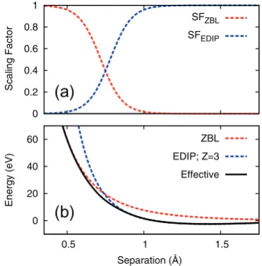
To accurately model close-ranged interactions between atoms, the pair potential within the EDIP formalism is smoothly switched to the ZBL pair potential[28]at small sep-arations. Due to the environmental dependence, this transi-tion is less straightforward than with pair potentials where interpolation functions such as cubic splines can be used to connect the potentials. Our approach uses two Fermi-type scaling functions (SFEDIP, SFZBL) which are defined using three

parameters; the positions of the midpoint of each function (rEDIP and rZBL) and the width w of the switching region.

After a trial-and-error process, values of rEDIP¼1:05 A˚ ,

rZBL¼0:45 A˚ , andw= 0.07 A˚ were selected to ensure a smooth

transition between the two regimes and to avoid inflexion points associated with changes in curvature. A plot of the switching functions along with the effective pair potential for a coordination number of three are shown inFig. 1. Note that this is the same approach as employed in previous EDIP simulations of ion impact[36,37]where the scaling function approach was first introduced and briefly defined.

Simulations were carried out in lattices equilibrated at 300 K and after the PKA was initiated the motion was followed for 5 ps. At the conclusion of the simulation steepest descent minimization was performed prior to defect analysis. Periodic boundary conditions were employed in each of the cartesian

0 20 40 60

0.5 1 1.5

Energy (eV)

Separation (Å)

(b)

ZBL

EDIP; Z=3

Effective 0

0.2 0.4 0.6 0.8 1

Scaling Factor

_(a)

SF_ZBL

SFEDIP

directions along with a 3.5A˚ thermal layer to remove excess kinetic energy during the cascade simulations. In addition, a layer of atoms perpendicular to the basal plane were held fixed to prevent any net transverse motion of the planes. To produce a representative set of collision cascades, a range of PKA energies and directions of initial velocity were sampled. Cascades were initiated with PKA energies of 100, 250, 500, 750, 1000, 1500, 2000 and 2500 eV within orthorhombic super-cells as large as 157.7·152.6·153.6 A˚3_{and containing up to}

440,448 atoms. As in the work of Robinson et al.[38], the ini-tial directions of the PKA were determined by uniformly dis-tributing points on a unit sphere (the so-called Thomson problem[39]) to select the direction of the initial velocity. This methodology allows for an arbitrary number of directions to be chosen. The data presented here is a composite of two uncorrelated data sets, one with 10 uniformly distributed data points and a second containing 20 points. To assist in retain-ing the cascade within the simulation cell, the location of the PKA atom was chosen such that the direction of initial motion was towards the center of the supercell.

Cascades were analysed using various quantitative mea-sures. The number of defects were computed using a vacancy radiusvrof 0.9 A˚ [40]. This value was also used to determine

atomic displacements. Coordination numbers are determined using a nearest-neighbor cutoff of 1.85 A˚ . At higher PKA ener-gies the graphite planes are prone to a degree of buckling due to the weak interlayer interactions. In a number of simula-tions this proved problematic, with significant numbers of atoms being identified as defects by the algorithm, even though their local environment was still purely graphitic. To circumvent this problem we added an additional criteria in which we computed the displacement perpendicular to the basal plane for all 3-fold coordinated atoms. If the magnitude of this displacement was less than 1.8 A˚ these atoms were identified as crystalline and removed from any subsequent defect analysis. Visual inspection of the problematic data sets showed that this approach worked extremely well, and meant the automatic defect counting algorithm could be used with confidence.

3.

Results

3.1. Individual cascades

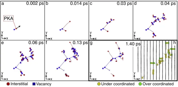
Fig. 2shows a representative example of a 1 keV cascade in

graphite. Blue squares denote vacancies while red circles denote interstitials. In the first frame (t= 0.002 ps) the PKA has moved on the order of the vacancy radius and has left behind a vacancy; the initial direction of the PKA is indicated by the arrow. After 0.014 ps the PKA has already experienced a close-approach collision with another carbon atom, effec-tively splitting into two sub-cascades. In the third and fourth frame (t= 0.03 and 0.04 ps) it is clear that the upper sub-cas-cade is the more energetic of the two and continues to exhibit a branching structure with each successive collision. In con-trast, the less energetic sub-cascade is already close to its end-of-range point. By 0.06 ps the entire cascade is close to maximum extent, with most of the remaining excess kinetic energy concentrated in a handful of atoms. At 0.13 ps the atoms no longer have sufficient energy to create new defects and self-induced annealing becomes the dominant process. The relaxation process is extremely rapid, and the structure at 1.40 ps is essentially identical to that when the simulation concludes. By this stage the number of defects has decreased considerably, from a peak of 37 interstitials at 0.11 ps, to 10 at 1.40 ps.

The final frame at the bottom-right of Fig. 2 shows an alternative view of the final structure, involving a rotation to highlight the cascade relative to the graphitic planes and a color-coding to indicate variations from the standard coordi-nation number of three. At the bottom left a single underco-ordinated atom results from the vacancy created by the PKA, while the green overcoordinated atoms mostly arise in the graphitic planes adjacent to an interstitial atom position between two-layers, thereby increasing the coordination number of the in-layer atoms to four. This is particularly apparent for the defect complex at the top of the panel where the yellow trajectory trace follows the path of the mobile atom which has moved between adjacent layers for a short

0.002 ps 0.014 ps 0.03 ps 0.04 ps

0.06 ps 0.13 ps _{1.40 ps}

a b c d

e f g h

Interstitial Vacancy Under coordinated Over coordinated x

y

x y

x y

x y

x y

x y

x y

z y

PKA

Fig. 2 – Typical cascade in graphite with a 1 keV primary knock-on atom (PKA). interstitials and vacancies are shown as red circles and blue squares respectively. For the time-series snapshots the atoms which remain on crystalline lattice sites are not shown. Panel (a) shows the system shortly after the PKA is initiated, while panel (g) is the final state. In the final image [panel (h)] atoms which are over- and under-coordinated (relative to the standard coordination of three forsp2_{hybridization)}

are shown as green and yellow spheres respectively. This is the same structure as the final state, differing only in the rotation of the view to highlight the graphitic planes shown in gray. (A color version of this figure can be viewed online.)

distance, eventually creating an interlayer defect. Density functional theory calculations[41] have identified a closely related configuration, known as the spiro interstitial due to its resemblance to the spiro-pentane molecule. Some of the structural details of the spiro interstitial (specifically, the two sets of triangular C–C bonds) differ to the MD simulation, but the origin of the discrepancy is well-known and arises from neglect of three-center terms, a common approximation in pair potentials and tight-binding methodologies[42]. The key observation is that the interlayer defect is indeed preva-lent in the simulations and is strongly correlated with over-coordinated atoms created by interstitials.

One of the striking features in Fig. 2 is the fractal-like branching structure of the defect trajectories. This arises from the highly energetic collisions involving the PKA and subsequently displaced lattice atoms. To convey a sense of the strength of these interactions we computed the maxi-mum kinetic energy of any atom, KEmax, and plotted this

quantity as a function of time (seeFig. 3). The arrows in the figure highlight the moments of close approach in which the PKA (or another more energetic atom) interacts strongly with an atom on a lattice site. At the instant of closest approach the velocities are transiently very small and the forces are enormous; the repulsion between the two atoms then splits the cascade and converts potential energy into kinetic energy spread between the two atoms. Correspond-ingly, each branching point seen in the time-series snapshots

of Fig. 2can be correlated to one of the close-approaches

denoted by the arrows inFig. 3.

Consideration of the details in Fig. 3 reveals an aspect which is initially surprising, namely, an extremely short time period when atoms have substantial kinetic energy. Cascade simulations in metals and oxides with PKA energies in the keV range typically evolve on the timescale of a picosecond or so, and yet here the maximum kinetic energy has fallen below 10 eV after just 0.090 ps. To quantify this behavior we counted the number of atoms with a kinetic energy exceeding thresholds of 1 and 10 eV. The latter is a measure of the num-ber of ‘‘fast atoms’’ which might be reasonably expected to be

associated with motion of atoms to a different lattice site or defect configuration, while the lower threshold conveys a sense of the rate at which the high thermal conductivity of the surrounding matrix removes heat from the cascade.

Fig. 4plots the time-dependence of both quantities and

con-firms the earlier impression fromFig. 3. The maximum num-ber of fast atoms (red trace) is achieved after just 0.032 ps, while the number of ‘‘warm atoms’’ (blue trace) first reduces to zero at 0.235 ps. These two quantities are indicated by arrows inFig. 4, and in preparation for later use we denote themtmaxandtend, respectively. This exceptionally rapid time

evolution is common to all cascades considered in this study and is quantified statistically in the following section. Given the striking difference compared to other materials, we calcu-lated the speed of sound in a diamond rod,[43]and repro-duced the known experimental value of around 12 km/s. This confirms that the rapid dynamics of the cascade is a bon-afide effect and highlights the value of studying graphite as a contrasting materials system as compared to the well-known radiation effects in metals and oxides.

On a technical level, the short-lived but highly energetic events inFigs. 3 and 4highlight the importance of the variable timestep algorithm. When the PKA is initiated the equations of motion are well-integrated using a timestep of 0.018 fs, but during the first collision this falls to just 0.0022 fs for a brief period, before increasing to a maximum of 0.025 fs mid-way between the first and second collisions. With each colli-sion the timestep is temporarily reduced and the cycle repeats, and the timestep gradually trends upwards towards a constant value of 0.23 fs by the end of the simulation. Across each collision the conservation of energy is excellent, leading to shifts no greater than 0.1 eV and typically far less. Due to the efficiency of the variable timestep algorithm, the total simulation of 5 ps was completed in fewer than 30,000 timesteps, with around 10,000 steps required to cover the first picosecond.

A second example of a 1 keV cascade in graphite is shown inFig. 5(a), this time employing a different initial PKA direc-tion. In this instance the cascade proceeds in a manner very different to that in Fig. 2. A branching structure is not

0 200 400 600 800 1000

0 0.02 0.04 0.06

KE

max

(eV)

time (ps)

Fig. 3 – Kinetic energy of the most energetic atom as a function of time in the 1 keV cascade inFig. 2. Vertical arrows indicate collisions with small impact parameters that transfer large amounts of kinetic energy to a lattice atom and effectively split the cascade into separate trajectories. (A color version of this figure can be viewed online.)

0 20 40 60 80

0 0.05 0.1 0.15 0.2 0.25 0.3

Number of atoms

time (ps)

t_max t_end

KE > 1 eV KE > 10 eV

Fig. 4 – Number of atoms with kinetic energy greater than 10 eV (red line) and 1 eV (blue line) in a 1 keV cascade as a function of time. Data applies for the cascade shown in Fig. 2. The arrows indicate two key cascade quantitiestmax

andtendas defined in the text. (A color version of this figure

observed, and instead the PKA is deflected into a channeling direction with a 10_{12 orientation. Once in the channel the}

PKA travels a substantial distance without creating perma-nent defects, losing energy at a constant rate of 18 eV per layer traversed. The kinetics of this process are summarized byFig. 5(b) which shows the time evolution of the most ener-getic atom in the cascade. Up until an end-of-range collision at 0.083 ps, the atom in question is always the PKA. Whilst in the channel the PKA undergoes a series of collisions in which it passes through the middle of a hexagonal ring of atoms, losing kinetic energy on entry and regaining a portion of this upon exit. Since the energy loss of 18 eV/layer is below the threshold displacement energy (which we show below to be around 25 eV), the disruption is transient and the lattice quickly recovers. The process is repeated nine times, during which the PKA travels more than 30 A˚ and loses around 160 eV without creating a single permanent defect.

The channeling direction along which the PKA travels is shown in ball-and-stick form in the inset withinFig. 5(b). It is immediately apparent that this is not a prototypical chan-nel such as found in a lattice with cubic symmetry, but instead a pseudo-channel in which the PKA must follow an undulatory path as it progresses through one layer to the next. We are not aware of this channeling direction having

previously been identified for graphite, a situation that per-haps reflects the difficulty of anticipating the pseudo-channel in the first place. Even for conceptually straightforward chan-nels such as those parallel or perpendicular to the c-axis, there are significant experimental difficulties associated with preparation of the sample and its alignment relative to the incident beam[44]. We return to this question of channeling in Section4where we discuss the simulations in the context of the historical literature.

3.2. Statistical analysis

Having outlined some of the qualitative features of radiation cascades in graphite, we now proceed to a quantitative treat-ment of various key properties. Statistical sampling is a cru-cial element of any cascade simulation analysis, and particularly so for graphite where the low packing fraction and anisotropic crystalline structure facilitates strong varia-tions in radiation response as a function and direction. Up to thirty directions are sampled for each PKA energy, provid-ing a high degree of precision which enables extraction of clear trends in the data.

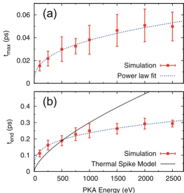
Fig. 6shows the energy dependence of the quantitiestmax

andtend defined inFig. 4. The solid points show the average

value while the error bars denote one standard deviation. The magnitude of the latter indicates the high degree of var-iability between individual cascade events and highlights the importance of sampling many uncorrelated directions. Due to the large number of simulations, the standard error in the mean is around a factor of 5 smaller than the ranges shown in the figure, and hence the solid points provide a good esti-mate of the true mean of both quantities. One of the surpris-ing facts to emerge fromFig. 6is the weak energy dependence

0 200 400 600 800 1000

0 0.02 0.04 0.06 0.08 0.1

KE

max

(eV)

time (ps) E=18 eV/layer

deflected into channel

a

b

Fig. 5 – (a) Snapshot for a 1 keV graphite cascade in which channeling occurs along ah1 0_{1 2idirection. The PKA was} initiated at the top-left of frame, traveling towards the bottom-right. (b) Maximum kinetic energy as a function of time. Green arrows indicate the collisions which deflect the PKA into the channel. Inset at top-right of panel denotes the pseudo-channels of graphite; blue and red circles represent the A and B planes, respectively. (A color version of this figure can be viewed online.)

0 0.1 0.2 0.3 0.4

0 500 1000 1500 2000 2500

tend

(ps)

PKA Energy (eV)

(b)

Simulation Thermal Spike Model 0

0.02 0.04 0.06

tmax

(ps)

(a)

Simulation Power law fit

Fig. 6 – (a) Dependence oftmaxas a function of PKA energy

wheretmaxis defined as the first time corresponding to the

highest number of fast atoms, i.e. KE > 10 eV. (b)

Dependence oftendas a function of PKA energy, wheretendis

defined as the first instant at which there are no ‘‘warm atoms’’ (i.e. atoms with KE > 1 eV). (A color version of this figure can be viewed online.)

of the time of peak defects (upper panel), and spike cooling time (lower panel). For example, increasing the PKA energy by a factor of four from 500 eV to 2 keV changestmaxby only

70% and tend by 55%. This behavior reflects the fractal-like

branching structure seen earlier inFig. 2where the cascade behavior is almost entirely ballistic, involving repeated split-ting into a series of sub-cascades. Accordingly, increasing the PKA by a large factor makes only a relatively small differ-ence to the cascade lifetime.

To quantify the difference between graphite cascades and those in most other materials we show in the lower panel of

Fig. 6the energy dependence for a thermal spike produced

when the energy of the PKA is delivered into a relatively com-pact region and induces local melting. Presuming a spherical spike for simplicity, an analytic solution[45]of the heat diffu-sion equation shows that the cooling time varies as E2=3_,

whereEis the PKA energy. This energy variation is shown as a solid black line inFig. 6, using the data point at 500 eV as an arbitrary anchor point. Clearly the graphite cascades have an energy dependence entirely unlike the thermal spike model, confirming the previous visual impressions seen in

Figs. 2 and 5that localised melting and extended disordering do not occur in graphite.

Having obtained these two numerical data sets, we subse-quently explored various mathematical functions, and found that both data sets are closely described by a power-law expression of the formaEx_{, wereEis the energy of the PKA.}

The fitted functions, shown as a blue-dotted line in each panel, reproduce the numerical data extremely well over a wide energy range, extending even to relatively low energies approaching the threshold displacement energy. For tmax,

which is the noisier of the two data sets due to smaller numerical values, the exponentx is 0.37, while for the cas-cade lifetimetendthe valuexis 0.28 and the fitting quality is

excellent. Since the exponent is so small, increasing the PKA energy to much larger values, for example, to 20 keV, only increases the spike lifetime by 80% relative to a 2.5 keV cas-cade. While we do not presently have a physical interpreta-tion for this power-law behavior, the quality of the fit is striking and it would be instructive to test the trend for much higher energies and to examine whether it can be exploited in simplified, non-MD, models of cascade evolution.

Fig. 7shows the energy dependence of the size of the cas-cade and the range of the PKA. The latter is determined by simply taking the difference between the initial and final positions of the PKA atom, while the cascade length is defined as the largest distance between any two defects in the cas-cade. For the purposes of this analysis, a defect was a defined as any atom with a local potential energy greater than7 eV/ atom. Since the cohesive energy of graphite in the EDIP for-malism is7.361 eV/atom, this corresponds to a strain energy of around 0.35 eV/atom. Visual inspection of the atoms iden-tified in this way showed this measure provided a simple and accurate measure of the region affected by the cascade. As in

Fig. 6, each data point is an average across as many as 30 dif-ferent directions and the error bars denote one standard devi-ation. Also shown inFig. 7are straight line fits to the two data sets. To a good approximation both the PKA range and cas-cade extent scale linearly with energy. The gradient of both quantities are quite similar, 27 A˚ /keV for the PKA range and

31 A˚ /keV for the cascade extent. For the highest energy cas-cade of 2.5 keV the PKA range is around 85% of the cascas-cade extent, and slightly smaller at lower energies. An immediate consequence of this linear variation is that increasing the PKA energy comes at high computational cost; numerical spe-cifics and possible alternative strategies are outlined in the Discussion.

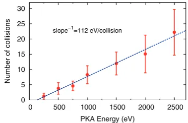
To quantify the process by which the PKA energy is con-verted into displacements we tracked the maximum kinetic energy KEmax in every simulation and analyzed its time

dependence. Motivated by data such as that shown inFig. 3, a collision was recorded if KEmax increased by more than

5 eV following a minimal value. This metric robustly identifies all of the heavy collisions indicated by arrows inFig. 3, as well as the much larger number of collisions for the channeling process inFig. 5. Once KEmaxbecomes sufficiently small, circa

50–100 eV, collisions are no longer identified since a subse-quent rise in kinetic energy does not occur following a close approach.

The results of the analysis are summarized inFig. 8, with the circles indicating the average number of collisions and the

0 20 40 60 80 100 120

0 500 1000 1500 2000 2500

Distance (

Å

)

PKA Energy (eV) Cascade Length

PKA Range

Fig. 7 – Cascade length (red) and PKA range (blue) as a function of PKA energy. Error bars denote one standard deviation, and the lines are linear fits to the data. For visual clarity, the data sets are offset slightly to the left and right of the relevant energy value. (A color version of this figure can be viewed online.)

0 5 10 15 20 25 30

0 500 1000 1500 2000 2500

Number of collisions

PKA Energy (eV)

slope1=112 eV/collision

Fig. 8 – Number of heavy collisions en-route to

thermalization as a function of PKA energy. The analysis employs KEmax(seeFig. 3) as discussed in the text. The blue

error bars indicating one standard deviation. The straight line is a linear fit to the data and intersects the average values with high accuracy; a companion plot employing the standard error of the mean is not shown as the resultant uncertainties are comparable in size to the circles used in the figure. Con-sidering a PKA energy of 1 keV as an example, we see that on average less than 10 collisions are required to thermalize the PKA, and that accordingly the branching cascade seen inFig. 2, with 9 collisions, is more typical than the channeling cascade (Fig. 5) which thermalizes after 19 collisions. From the inverse slope of the linear fit to the data we see that a typ-ical collision loses 112 eV, a result which is consistent with visual inspection of the branching cascade. The linear behav-ior holds over the entire energy range considered, and makes a useful starting point for estimating the behavior of more energetic cascades.

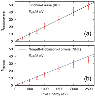
Two of the most crucial quantities to quantify in a radia-tion cascade simularadia-tion are the number of displaced atoms and the number of defects created. As noted in Section 2, we define defects and displacements using a vacancy radius of 0.9 A˚ . The energy dependence of both data sets is shown

in Fig. 9, along with the theoretical behavior predicted by

the Kinchin–Pease (KP) [46] and Norgett–Robinson–Torrens (NRT) [47] models. Both models employ the threshold dis-placement energy,Ed, as a single parameter; in the KP model

the number of displacements is computed asE=ð2EdÞ, whereE

is the PKA energy, while in the modification of NRT an addi-tional multiplicative factor of 0.8 is included to empirically describe recombination. Consistent with the experimental and computational literature, a value of Ed¼25 eV was

assumed for the two models. The simulations show excellent correlation with the two theories, a result which is somewhat remarkable in itself given that the theoretical underpinnings of the KP and NRT treatments are not especially strong,

especially regarding the NRT factor of 0.8 which dates back to a computer simulations performed in the mid 1970’s. In many metal and oxide systems defect recombination in the post-ballistic phase can lead to vastly fewer defects than displacements, and hence the KP/NRT methods don’t always provide predictive power. For graphite, however, these simple models work extremely well, even down to the empirical factor of 0.8 which relates displacements to defects.

4.

Discussion and conclusion

One of the main insights to emerge from this study is the pro-found difference between cascades in graphite as compared to other widely-studied solids. The branching structure, absence of localized melting, and KP-type defect generation are all examples of behavior which place graphite in a special category. Equally interesting is that many of these insights were correctly qualitatively understood long ago, as demon-strated byFig. 10, which compares two literature schematics of cascades from fast neutron damage in graphite [panels

(a)

(b)

Fig. 9 – Number of displacements [panel (a)] and defects [panel (b)] as a function of PKA energy. Error bars indicate the standard deviation. Defects are identified using a vacancy radius of 0.9 A˚ . The solid lines show the Kinchin– Pease and Norgett–Robinson–Torrens relationships assuming a threshold displacement energy,Ed, of 25 eV. (A

color version of this figure can be viewed online.)

a

b

c

PKA

2.5 keV

Vacancy Interstitial

Fig. 10 – Comparison between literature models of graphite radiation damage and simulations performed in this work. The dotted boxes in the upper schematics have been added to highlight the cascade portion within the diagram. (a) Schematic from Nightingale (p. 213 in[48]). (b) Schematic from Simmons (p. 20 in[49]), (c) Cascade simulation for a PKA energy of 2.5 keV. Schematics reprinted with permis-sion from Elsevier. (A color verpermis-sion of this figure can be viewed online.)

(a,b)] with a 2.5 keV simulation from this work [panel (c)]. Both schematics date from the 1960’s, with panel (a) from Nightingale[48]and panel (b) from Simmons[49]. Although one could argue the minor details of the schematics, the broad picture is clearly correct, particularly regarding the branching structure of the trajectories. As for the origin of this behavior, a definitive answer cannot yet be given, but possible reasons include the low mass of carbon relative to many solids, the high thermal conductivity of graphite, and the low-packing fraction. All of these ideas are amenable to computer simulation through controlled comparison studies, and represent a promising direction for future work.

Where the simulations offer a clear advance over previous empirical understanding is in quantitation. Key quantities such as the threshold displacement energy, PKA range, mean free path, etc, have been subject to considerable uncertainty. In the case of the range of the PKA, Simmons[49]quotes a value of 67 A˚ for a 1 keV PKA, as compared to the 30 A˚ com-puted here. The same source similarly overestimates energy loss per collision, listing a value of 196 eV per collision as compared to our value of 112 eV per collision. Earlier hard-sphere results reported in Nightingale[48]disagree to an even larger extent, predicting a mean-free-path between collisions of 84 A˚ for a 1 keV PKA. EstablishingEdfor graphite has also

been highly problematic, with literature estimates covering a wide range, spanning 10 to 60 eV [50,51]. In contrast, our value of 25 eV determined by the KP and NRT relationships is statistically sound. Burchell has previously noted[52]that a value of 60 eV has gained wide acceptance (specifically in the nuclear industry) but argues that a much smaller value of 30 eV is appropriate; the estimate here of 25 eV is broadly consistent with this assessment. We note that Yazyev et al.

[9]also estimated anEdvalue of 25 eV from their density

func-tional theory calculations, while Smith and Beardmore [8]

reported 34.5 eV, and Hehr et al.[10]reported around 45 eV. As a caveat, we note that direct analysis of MD trajectories (such as in [38]can provide an even more refined estimate ofEd, and so the present number should not be considered

the final value. Such an approach is the most unambiguous route to determiningEd, since the analysis is based entirely

on counting statistics over a large number of trajectories, and no inputs or prior functional form need to be assumed, save the interatomic potential itself.

Regarding channeling, there have been a few experimental studies[44,53], but the measurements are difficult and sam-ple preparation and alignment are paramount. Channeling down ah0 0 0 1ichannel (i.e. parallel to thec-axis) has been observed (seeFig. 1in[53]for a schematic), and long ago it was proposed [54] that channeling might occur in the

h1 12 0idirection. The simulations show that while channel-ing is not a common occurence, it is certainly possible under certain conditions. To the best of our knowledge the channel-ing process shown inFig. 5has not been previously described or envisaged and is an excellent example how computer sim-ulation can provide new insights into radiation phenomena. The closest connection with previous work is the calculation of Kaxiras and Pandey[55]which found that a hexagon center defect in graphite has an energy of 19.5 eV, close to the energy loss rate observed in the simulations, suggesting that the PKA has to climb up the potential hill of 18 eV before being

squeezed out again. Finally, we note that one of the factors which limits channeling is that the atoms are invariably ini-tially located on a lattice site and hence displacement tends to cause an immediate collision with a nearby atom. A differ-ent situation exists for interstitial carbons, but such atoms are present in low numbers and cannot be considered typical. Looking to future simulations of cascades in graphite, sev-eral conclusions immediately present themselves. Firstly, there are promising prospects to study how temperature affects the evolution of the cascade and the associated relax-ation dynamics. As discussed by Kelly[56], a large experimen-tal literature exists for graphite on dimensional change, mechanical behavior and thermal properties. However, simu-lations have not been applied to the atomistic perspective. It would be particularly fruitful to combine defect analysis as carried out in this work with density functional theory calcu-lations of defect energetics and activation barriers for migra-tion and recombination. This knowledge would be particularly beneficial for understanding graphite structural evolution under irradiation such as the recently proposed ruck-and-tuck model [57]. On a technical level, one unex-pected detail is that wall thermostats are not essential as the simulation cells are sufficiently large that the excess kinetic energy of the PKA is easily accommodated within the cell. For the simulations performed here, the excess energy was typically 0.005 eV/atom and hence the tempera-ture rise is of the order tens of Kelvin. More significant is the very large number of atoms required to contain the cas-cade as the PKA energy rises. Extrapolating the data inFig. 7

to higher energies shows that very large simulation cells are required to reliably avoid the cascade interacting with the boundaries. To contain a 5 keV cascade at a 2r confidence level (97.5%) requires a cell of 2 million atoms; the required supercell side-length is 263 A˚ , comprising 253 A˚ from the extrapolation of the mean cascade length plus two standard deviations, and a boundary layer of 10 A˚ . Higher energies make the numerics even more extreme, as the number of atoms required scales asE3due to the linear variation shown inFig. 7. For example, 40 keV cascades have been simulated in a variety of oxides[58], but the same calculations in graphite would require 1 billion atoms, far beyond what is presently practicable for carbon. For large systems it may be preferable instead to develop a stochastic approach based upon the atomistically-derived information extracted from molecular dynamics. Such a scheme should in-principle be possible given the high statistical reproducibility evident in the com-putational data presented here.

well as providing a starting point for future studies of defect generation under irradiation. This information is invaluable for understanding the role of graphite under irradiation, a topic of great importance for lifetime extension of existing nuclear reactors and next-generation designs operating at high temperature.

Acknowledgments

The project used advanced computational resources provided by the iVEC facility at Murdoch University. Discussions with Malcolm Heggie and Alice McKenna are acknowledged. HJC, DLR and DKR thank the Engineering and Physical Sciences Research Council and the Technology Strategy Board for their support through Grants EP/I003312/1 and 101437, respectively. ISM and NAM thank the Australian Research Council for fel-lowships, and MR thanks the Australian Nuclear Science and Technology Organisation for support.

R E F E R E N C E S

[1]Weber WJ, Ewing RC, Catlow CRA, Diaz de la Rubia T, Hobbs L, Knoshita C. Radiation effects in crystalline ceramics for the immobilization of high-level nuclear waste and plutonium. J Mater Res 1998;13:1434.

[2]Nordlund K, Ghaly M, Averback RS, Caturla M, Diaz de la Rubia T, Tarus J. Defect production in collision cascades in elemental semiconductors and fcc metals. Phys Rev B 1998;57(13):7556.

[3]Bacon DJ, Gao F, Osetsky YN. Computer simulation of displacement cascades and the defects they generate in metals. Nucl Instrum Meth B 1999;153(1):87–98.

[4]Bacon DJ, Gao F, Osetsky YN. The primary damage state in fcc, bcc and hcp metals as seen in molecular dynamics simulations. J Nucl Mater 2000;276(1):1–12.

[5]Marks NA. Computer-based modeling of novel carbon

systems and their properties: beyond nanotubes. Springer; 2010.

[6]Ewels C, Telling R, El-Barbary A, Heggie M, Briddon P. Metastable Frenkel pair defect in graphite: source of Wigner energy? Phys Rev Lett 2003;91(2):025505.

[7]Telling RH, Heggie MI. Radiation defects in graphite. Philos Mag 2007;87(31):4797–846.

[8]Smith R, Beardmore K. Molecular dynamics studies of particle impacts with carbon-based materials. Thin Solid Films 1996;272(2):255–70.

[9]Yazyev OV, Tavernelli I, Rothlisberger U, Helm L. Early stages of radiation damage in graphite and carbon nanostructures: a first-principles molecular dynamics study. Phys Rev B 2007;75(11):115418.

[10]Hehr BD, Hawari AI, Gillette VH. Molecular dynamics simulations of graphite at high temperatures. Nucl Technol 2007;160(2):251–6.

[11] Neighbour GB, editor. Management of ageing in graphite reactor cores. Cambridge, UK: The Royal Society of Chemistry; 2007.http://dx.doi.org/10.1039/9781847557742. [12] Haller J.<http://www.euronuclear.org/events/enc/enc2012/

transactions/ENC2012-transactions-plant-operations.pdf>

[accessed 20.05.2014].

[13] Technology Roadmap Update for Generation IV Nuclear Energy Systems,<https://www.gen-4.org/gif/upload/docs/ application/pdf/2014-03/gif-tru2014.pdf>[accessed 20.05.2014].

[14] Gibson JB, Goland AN, Milgram M, Vineyard GH. Dynamics of radiation damage. Phys Rev 1960;120(4):1229.

[15] Daw MS, Baskes MI. Semiempirical, quantum mechanical

calculation of hydrogen embrittlement in metals. Phys Rev Lett 1983;50(12):1285.

[16] Daw MS, Baskes MI. Embedded-atom method: derivation and

application to impurities, surfaces, and other defects in metals. Phys Rev B 1984;29(12):6443–53.

[17] Lewis GV, Catlow CRA. Potential models for ionic oxides. J Phys C Solid State 1985;18(6):1149–61.

[18] Bush TS, Gale JD, Catlow CRA, Battle PD. Self-consistent interatomic potentials for the simulation of binary and ternary oxides. J Mater Chem 1994;4(6):831–7.

[19] Lumpkin GR, Smith KL, Blackford MG, Thomas BS, Whittle

KR, Marks NA, et al. Experimental and atomistic modeling study of ion irradiation damage in thin crystals of the TiO2 polymorphs. Phys Rev B 2008;77(21):214201.

[20] Smith R. A classical dynamics study of carbon bombardment of graphite and diamond. Proc R Soc Lond A

1990;431(1881):143–55.

[21] Tersoff J. Empirical interatomic potential for carbon, with applications to amorphous carbon. Phys Rev Lett 1988;61(25):2879–82.

[22] Brenner DW. Empirical potential for hydrocarbons for use in simulating the chemical vapor deposition of diamond films. Phys Rev B 1990;42(15):9458–71.

[23] Heggie MI. Semiclassical interatomic potential for carbon and its application to the self-interstitial in graphite. J Phys Condens Mater 1991;3(18):3065.

[24] Nordlund K, Keinonen J, Mattila T. Formation of ion irradiation induced small-scale defects on graphite surfaces. Phys Rev Lett 1996;77(4):699–702.

[25] Krasheninnikov AV, Nordlund K. Ion and electron irradiation-induced effects in nanostructured materials. J Appl Phys 2010;107(7):071301.

[26] Marks NA. Generalizing the environment-dependent

interaction potential for carbon. Phys Rev B 2001;63(3):035401. [27] Marks N. Modelling diamond-like carbon with the

environment-dependent interaction potential. J Phys Condens Mater 2002;14(11):2901–27.

[28] Ziegler JF, Biersack JP, Littmark U. The stopping and range of ions in solids, vol. 1. New York: Pergamon; 1985.

[29] Lau DWM, McCulloch DG, Marks NA, Madsen NR, Rode AV.

High-temperature formation of concentric fullerene-like structures within foam-like carbon: experiment and molecular dynamics simulation. Phys Rev B 2007;75(23):233408.

[30] Powles RC, Marks NA, Lau DWM. Self-assembly of sp2 -bonded carbon nanostructures from amorphous precursors. Phys Rev B 2009;79:075430.

[31] Suarez-Martinez I, Marks NA. Effect of microstructure on the thermal conductivity of disordered carbon. Appl Phys Lett 2011;99(3):033101.

[32] Suarez-Martinez I, Higginbottom PJ, Marks NA. Molecular dynamics simulations of the transformation of carbon peapods into double-walled carbon nanotubes. Carbon 2010;48(12):3592–8.

[33] Suarez-Martinez I, Marks NA. Amorphous carbon nanorods

as a precursor for carbon nanotubes. Carbon 2012;50(15):5441–9.

[34] Marks NA, Lattemann M, McKenzie DR. Nonequilibrium

route to nanodiamond with astrophysical implications. Phys Rev Lett 2012;108(7):075503.

[35] Justo JF, Bazant MZ, Kaxiras E, Bulatov VV, Yip S. Interatomic potential for silicon defects and disordered phases. Phys Rev B 1998;58(5):2539–50.

[36] Marks NA, Bell JM, Pearce GK, McKenzie DR, Bilek MMM. Atomistic simulation of energy and temperature effects in

the deposition and implantation of amorphous carbon thin films. Diamond Relat Mater 2003;12(10–11):2003–10.

[37]Pearce GK, Marks NA, McKenzie DR, Bilek MMM. Molecular

dynamics simulation of the thermal spike in amorphous carbon thin films. Diamond Relat Mater 2005;14(3–7):921–7. [38]Robinson M, Marks NA, Whittle KR, Lumpkin GR. Systematic

calculation of threshold displacement energies: case study in rutile. Phys Rev B 2012;85(10):104105.

[39]Thomson JJ. On the structure of the atom. Philos Mag 1904;7:237.

[40] The vacancy radius is empirically determined, but in practice it is restricted to a relatively small range. Values of 0.7 A˚ , similar to the covalent radius, overestimate the number of defects, specifically split interstitials where the midpoint of the bond is located at the original lattice site. Values larger than 1.1 A˚ underestimate defects, in particular vacancies where structural relaxation occurs around the empty lattice site. The value of 0.9 A˚ is an appropriate middle-ground between the two extremes, as confirmed by visual comparison between defect structures arising during cascades and those automatically identified via the vacancy radius.

[41]Telling RH, Ewels CP, El-Barbary AA, Heggie MI. Wigner defects bridge the graphite gap. Nat Mater 2003;2(5):333–7. [42]Marks NA, Cooper NC, McKenzie DR, McCulloch DG, Bath P,

Russo SP, et al. Comparison of density-functional, tight-binding, and empirical methods for the simulation of amorphous carbon. Phys Rev B 2002;65(7):075411.

[43] The test on diamond is a validation of the fundamentals of the molecular dynamics package. The speed of sound in graphite is difficult to access (either via simulation or in the laboratory) due to the weak interlayer interaction and crystalline imperfections. In contrast, the diamond structure is straightforward to study from both a computational and experimental point of view, and therefore provides the most straightforward route for low-level verification.

[44]Elman BS, Braunstein G, Dresselhaus MS, Dresselhaus G, Venkatesan T, Wilkens B. Channeling studies in graphite. J Appl Phys 1984;56(7):2114.

[45]Marks NA. Evidence for subpicosecond thermal spikes in the formation of tetrahedral amorphous carbon. Phys Rev B 1997;56(5):2441–6.

[46]Kinchin GH, Pease RS. The mechanism of the irradiation disordering of alloys. J Nucl Energy 1954;1(2–4):200–2. [47]Norgett MJ, Robinson MT, Torrens IM. A proposed method of

calculating displacement dose rates. Nucl Eng Des 1975;33(1):50–4.

[48]Nightingale RE, editor. Nuclear graphite. New York and London: Academic Press; 1962.

[49]Simmons JHW, editor. Radiation damage in graphite. Pergamon Press; 1965.

[50]Zinkle SJ, Kinoshita C. Defect production in ceramics. J Nucl Mater 1997;251:200–17.

[51]Banhart F. Irradiation effects in carbon nanostructures. Rep Prog Phys 1999;62(8):1181–221.

[52]Burchell TD, editor. Carbon materials for advanced technologies. American Carbon Society; 1994.

[53]Yagi E, Iwata T, Urai T, Ogiwara K. Channelling studies on the lattice location of B atoms in graphite. J Nucl Mater 2004;334(1):9–12.

[54]Balarin M. Focusing conditions for elastic atomic collisions in graphite (in german). Phys Status Solidi 1962;2:60.

[55]Kaxiras E, Pandey KC. Energetics of defects and diffusion mechanisms in graphite. Phys Rev Lett 1988;61(23):2693. [56]Kelly BT, editor. Physics of graphite. Applied Science

Publishers; 1981.

[57]Heggie MI, Suarez-Martinez I, Davidson C, Haffenden G. Buckle, ruck and tuck: a proposed new model for the response of graphite to neutron irradiation. J Nucl Mater 2011;413:150–5.