A physically constrained source model for FDTD acoustic simulation

A physically­constrained source model for 

FDTD acoustic simulation

Sheaffer, J, Walstijn, MV and Fazenda, BM

Title

A physically­constrained source model for FDTD acoustic simulation

Authors

Sheaffer, J, Walstijn, MV and Fazenda, BM

Type

Conference or Workshop Item

URL

This version is available at: http://usir.salford.ac.uk/id/eprint/23028/

Published Date

2012

USIR is a digital collection of the research output of the University of Salford. Where copyright 

permits, full text material held in the repository is made freely available online and can be read, 

downloaded and copied for non­commercial private study or research purposes. Please check the 

manuscript for any further copyright restrictions.

A PHYSICALLY-CONSTRAINED SOURCE MODEL FOR FDTD ACOUSTIC SIMULATION

Jonathan Sheaffer,

Acoustics Research Centre

School of Computing, Science and Engineering

University of Salford

Salford, UK

[email protected]

Maarten Van Walstijn,

Sonic Arts Research Centre

School of Electronics, Electrical Engineering,

and Computer Science. Queen’s University Belfast

Belfast, UK

[email protected]

Bruno Fazenda,

Acoustics Research Centre

School of Computing, Science and Engineering

University of Salford

Salford, UK

[email protected]

ABSTRACT

The Finite Difference Time Domain (FDTD) method is becoming increasingly popular for room acoustics simulation. Yet, the lit-erature on grid excitation methods is relatively sparse, and source functions are traditionally implemented in ahardoradditiveform using arbitrarily-shaped functions which do not necessarily obey the physical laws of sound generation. In this paper we formu-late a source function based on a small pulsating sphere model. A physically plausible method to inject a source signal into the grid is derived from first principles, resulting in a source with a near-flat spectrum that does not scatter incoming waves. In the final discrete-time formulation, the source signal is the result of passing a Gaussian pulse through a digital filter simulating the dynamics of the pulsating sphere, hence facilitating a physically correct means to design source functions that generate a prescribed sound field.

1. INTRODUCTION

The FDTD method has recently become more popular for room acoustics simulation, very much owing to the increased process-ing power and memory resources of more commonly available computing hardware. This is evident in newly emerged numer-ical schemes [1, 2] and optimised parallel implementations [3], which provide means for more accurate and efficient modelling. In room-acoustics FDTD, one wishes to correctly excite a 3D grid for simulation of longitudinal acoustic wave propagation, which is a different challenge than excitation of other grids, for example for simulating transversely vibrating mechanical systems [4].

Traditionally, excitation functions are either imposed or super-imposed onto the source occupying node. The former method is often referred to as ahard sourceinjection where the pressure at the source position is directly set by the excitation function and the update equations for the acoustic medium are bypassed. The lat-ter approach, often referred to as asoft source, describes a method in which the excitation function is added to the existing pressure at the source position, which has already been evaluated by the medium update equations.

Hard sourcesare common, most likely due to their simplicity and ease of implementation. However, the imposition of pressure directly on the grid is artificial and bears some complications. It suggests that acoustic pressure appears with no underlying phys-ical cause, and as such, does not obey the laws of fluid dynam-ics. As the hard-source node scatters incoming waves, it can be loosely thought of as a sound radiating boundary node whose size corresponds to the spatial sample period. This characterisation, however, is also not precise, as such elements should adhere to boundary conditions which are not evident in the hard source for-mulation. For simulation of enclosed spaces, scattering caused by the hard-source node is artificial and detrimental to the result. Even when boundary reflections do not occur some artefacts may arise. Since the hard source is directly imposed on the grid, the transient change in sound pressure at the source node takes the form of the source function, which is a desired feature, as one can directly employ excitation signals that generate a prescribed pressure. However, as the equations of mass and momentum are not satisfied at the source node, the inability of air particles to ef-fectively perform rarefaction may cause unwanted low-frequency artefacts when certain excitation signals are used [5]. Thus, we postulate that the hard source paradigm is fundamentally flawed in the sense that it does not adhere to any physical laws governing the medium or the boundaries.

The source-scattering and low-frequency problems can be over-come by employingSoft Sources. In such case, the excitation func-tion is superimposed on the pressure at the source node, which causes it to be modified by the grid’s impulse response [6]. Fur-thermore, in Yee-based schemes [7] the source function is differ-entiated by the staggered update equation, causing a steep roll-off at low frequencies. For schemes based on the wave equation, Kar-jalainen and Erkut [8] have shown that additive sources should be equivalently filtered withH(z) = 1−z−2

, which generates the same effect.

ap-proach requires that the grid’s impulse response is measured prior to the simulation stage and compensated for during simulation. Therefore, it is more computationally expensive and less intuitive to implement. Furthermore, it has been shown that transparent sources also suffer from the same low frequency artefacts as hard sources [5].

Another concern which has not been thoroughly explored in context of multidimensional schemes, is the relation of the source magnitude to the numerical properties of the grid. When the ampli-tude of the excitation function is arbitrarily chosen, the magniampli-tude of the resulting pressure field varies with sample rate. Due to the Courant criterion, the temporal sample-rate controls the physical volume of each grid cell, which must be taken into account when scaling the source signal.

In this paper we address all of these issues by introducing an integrated source excitation approach which adheres to both phys-ical and numerphys-ical constraints, and is derived entirely from first principles. The source function is based on a theoretical point-monopole governed by a force-driven mass-damper-spring sys-tem. This mechanism conceptually resembles the output of an electro-mechanical transducer with an omnidirectional sound radi-ation pattern. We then show how a source can be embedded in an FDTD grid by discretising the appropriate fluid-dynamic govern-ing equations. This results in anadditivesource injection method which is correctly scaled with FDTD parameters and is in agree-ment with analytic solutions to the wave equation. The entire sys-tem is represented as a set of DSP operations, which can be used to generate a prescribed pressure source function of near-flat spec-trum within a controlled bandwidth.

Section 2 discusses the governing equations in the mechanical and acoustical domains. Section 3 provides a numerical formula-tion of the method, for both synthesising a source signal and in-jecting it into an FDTD grid. Results for some typical applications are shown in Section 4, followed by a discussion and conclusions.

2. GOVERNING EQUATIONS 2.1. Sound Source

We consider a pulsating sphere of (small) radiusa0whose surface

velocityu(t), in vacuum, is governed by

M∂u(t)

∂t =−Ru(t)−K

Z

u(t)dt+F(t) (1)

whereM,R, andKare respectively, the mass, damping and elas-ticity constants characterising the mechanical system, andF(t)is the force driving the sphere pulsation. With air surrounding the sphere, the mechanical impedance of the system is

Z(ω) =Zv(ω) +Za(ω) (2)

whereZv(ω) =M jω+R+K/(jω)is the impedance of the sys-tem in vacuum andZa(ω) =ρ0Aa0 jω−(a0/c)ω2

is the me-chanical impedance of the surrounding air [9, p. 315]. However, the latter term may be omitted sincea0is very small, meaning that

|Zv(ω)|>>|Za(ω)|in all practical cases. Hence the system may be characterised by the transfer function

H(s) = 1

M s+R+K/s (3)

which has the dimension of mechanical admittance. In the time domain, the impulse response of the system is given by

h(t) = 1

M eαt

cos(ωrt)− α ωr

sin(ωrt)

(4)

whereα = R

2M is the damping factor,ω0 =

q

K

M is the sys-tem’s undamped resonant frequency andωr =

p

ω2

0−α2. At

the source, the sphere’s surface velocity equals the particle ve-locity of air, which can be mathematically expressed as convolu-tion between the driving force and the system’s impulse response, u(t) = F(t)∗h(t). The pulsation of the sphere causes fluid to be pushed into and extracted from the region bordering the source sphere surface, which is characterised by avolume velocity,

ˆ

q(t) =u(t)As (5) having the dimensions of volume per unit time (m3_s−1_{), where}

As= 4πa20is the surface area of the sphere.

2.2. Sound Generation and Propagation

The conceptual point-monopole described in section 2.1 generates a volume velocityqˆ(t)at the source position. We shall now relate this quantity to the inhomogeneous wave equation,

1

c2

∂2_p(

x, t)

∂t2 − ∇ 2

p(x, t) =ψ(x, t) (6) which is used to describe the sound field atx= (x, y, z) ∈R3.

In order to enable direct comparison with other studies, we de-fineψ(x, t)as a general source driving function which can take on any form or shape. In this section we aim to derive an appro-priateψwhich will obey the physical laws of fluid emergence, by first considering the conservation laws of mass and momentum. In their Eulerian form, the continuity and momentum equations with sources are given by [9, p. 241]

∂ρ(x, t)

∂t +ρ0∇ ·u(x, t) =q(x, t) (7) ρ0

∂u(x, t)

∂t +∇p(x, t) =Fe(x, t) (8) Whereρ0 is the ambient density of air, ρ(x, t) is the transient

change of density, andu(x, t)andp(x, t)are the particle velocity and pressure respectively. Here, the functionq(x, t)denotes the rate of fluid emergence in the system in the dimensions of density per unit time (kg m−3s−1), and the functioneF(x, t)is the

acous-ticforce exerted upon the source volume (not to be confused with the mechanical force driving the sphere pulsation). In the prob-lem discussed in this paper, the sound source is considered to be an acoustic transducer converting mechanical forces into volume velocity. Therefore, it is reasonable to treatq(x, t)as the primary source generating function, and the force term in equation (8) is neglected. Considering now a source positioned at a single node of an FDTD grid, in which each cell occupies a volume equal to X3, we can relate the volume velocity of the sourceqˆ(t)to the source density termq(x, t)as follows

q(x, t) = ρ0

X3qˆ(t)δ(x−x

0

) (9)

wherex0= (x0, y0, z0)∈R3denotes the source position. As will

(9) results in correct magnitude scaling of the source signal. To ex-press equation (7) as a function of acoustic ex-pressure, it is assumed thatkuk cand the equation of statep(x, t) =c2ρ(x, t)can be used to convert density to pressure, yielding

∂p(x, t)

∂t =−ρ0c

2_{∇ ·}

u(x, t) +c2q(x, t) (10) By combining equations (8) and (10), the particle velocity vector is eradicated and the wave equation (6) is derived (note that here equation (8) is used without the acoustic force term). It follows from this derivation that the source term becomes

ψ(x, t) =∂q(x, t)

∂t = ρ0

X3

d

dtqˆ(t)δ(x−x 0

) (11)

Physically, the quantityψ(x, t)has the dimensions of density per unit time squared (kg m−3 _s−2_{), and can be thought of as fluid}

emergence due to volume acceleration of the source.

In a spherically-symmetrical system, an analytic solution for (6) in free field is possible. In such case, the spherical Laplace op-erator in (6) becomes angle-independent, and with a point-source approximation, the sound pressure at the distancer=kx−x0kis given by [9, p. 310]

p(r, t) = ρ0 4πr

d dtqˆ

t−r

c

(12)

For qˆ(t) = δ(t−t0), equation (12) is the transient free-field Green’s function solution to the wave equation.

3. NUMERICAL FORMULATION

In this section we present the proposed source formulation in the numerical domain. Here it is applied to a family of schemes for the wave equation which have been shown to be efficient in simulating room acoustics [1]. A similar formulation is possible for other schemes.

3.1. Compact Explicit Schemes

The wave equation (6) can be modelled using centred finite differ-ence (FD) operators as

δt2−λ

2

δx2

pni =c 2

T2ψin | {z } Source Term

(13)

whereX is the spatial sample period,T is the temporal sample period,λ=cT /Xis the Courant number, and the pressure field is discretised such that

p

n

i =p(x, y, z, t)

x=lX,y=mX,z=iX,t=nT (14) The discrete FD operators are given by

δt2p n

i ≡p

n+1

i −2p

n

i +p

n−1

i (15)

δx2p n

i ≡p

n

l+1,m,i−2p

n l,m,i+p

n

l−1,m,i (16) δy2p

n

i ≡p

n

l,m+1,i−2p

n l,m,i+p

n

l,m−1,i (17) δz2p

n

i ≡p

n

l,m,i+1−2p

n l,m,i+p

n

l,m,i−1 (18)

where the spatial index vectoriand operatorδ2

x are given by

i= [l, m, i] (19)

δ2x =δ 2

x+δ

2

y+δ

2

z+a δ

2

xδ

2

y+δ

2

xδ

2

z+δ

2

yδ

2

z

+bδx2δ

2

yδ

2

z (20) The free parametersaandbare chosen according to the desired numerical properties, which fora= 0, b= 0results in the well knownstandard rectilineargrid. For the source node, the driving functionψis given in the discrete domain by

ψni0 = ρ0

X3_2T

ˆ

q

n+1

−qˆ

n−1

(21)

and accordingly, equation (13) can be expressed in additive form as follows

p

n+1

l0_,m0_,i0 = n

p

n+1

l0_,m0_,i0 o

+ρ0cλ 2X2

ˆ

q

n+1

−qˆ

n−1

(22)

wherep

n+1

l0_,m0_,i0is the pressure at the source node and n

p

n+1

l0_,m0_,i0 o

represents the result of updating the node with the regular air up-date equation (see Appendix I). The apostrophe symbols above spatial indices denote that the equation is evaluated at the source node.

3.2. Representation in the Z-Domain

In the discrete domain, equation (22) requires that the volume ve-locity,qˆ

n

is obtained fromu

n

. This function can be generated by discretising the convolution of a specified driving forceF(t)

with the impulse response of the system (4). However, we may represent the system directly in the z-domain, avoiding the need to explicitly perform convolution in the time-domain. Here we opt to apply the bilinear transform in order to obtain the z-domain trans-fer function of the system. This choice is mainly because, unlike other discretisation methods, the bilinear transform does not place any stability limits on the values ofM,RandK, thus allowing them to be freely chosen. The bilinear transform of equation (3) is

H(s)

s=β1−z−1

1+z−1

= (23)

β 1−z−2

(M β2_{+Rβ+K) + (2K−2M β}2_)z−1_{+ (M β}2_−Rβ+K)z−2

whereβ is the bilinear operator, which for a pre-warpedω0 is

given by

β= ω0 tan(ω0T /2)

(24)

Normalising (23) we can express the system in a form of a digital filter

H(z) = b0+b2z

−2

1 +a1z−1+a2z−2

(25)

With the coefficients given by

b0 =

β

M β2_+Rβ+K (26)

b2 = −

β

M β2_+Rβ+K (27)

a1 =

2 K−M β2

M β2_+Rβ+K (28)

a2 = 1−

2Rβ

M β2_+Rβ+K (29)

In the discrete domain, a driving forceF

n

Figure 1: DSP block diagram of source generation and injec-tion. F

n

denotes driving force,H(z)is the transfer function of the point-monopole model,u

n

denotes surface velocity,q

n

de-notes the rate of fluid emergence in the system,ψ

n

denotes the source function,{p

n+1

i’ }is the regular update equation for air,

andp

n+1

i’ is the resulting sound pressure at the source node.

byρ0As/X3to directly obtainq

n

i0. The complete signal

process-ing required for generatprocess-ing and injectprocess-ing the source into the grid is graphically shown in figure 1. Note that the processing shown in figure 1 outputs a signal which is delayed by one-sample in com-parison to the result of equation (22). In this paper we refer to the entire model presented here as aPhysically-Constrained Source, abbreviatedPCShereafter.

4. RESULTS 4.1. Prescribed Pressure Source

In room acoustics simulation, it is desirable to design a source function that generates a prescribed sound field. In this section we show how thePhysically-Constrained Source(PCS) can be used to accomplish this task. The goal is to design an excitation signal that propagates omni-directionally and has a flat frequency response within a defined frequency range. It is not possible (nor phys-ically practical) to implement a source mechanism with infinite bandwidth. Nevertheless, some properties of the system can be exploited to effectively band-limit the excitation signal whilst still maintaining a near-flat frequency response within its passband.

The low-frequency behaviour of the source is characterised by the system resonanceω0and quality factorQ. The former controls

the low cut-off frequency whilst the latter defines the steepness of the transition between the rolled-off frequencies and the pass-band. In an optimal transducer design process, the designer would specify the desired values for these parameters and the remaining electro-mechanical quantities would be engineered accordingly. In the model presented herein, it is assumed that the source has some mass,M, and the remaining damping and stiffness coefficients are then calculated fromR = ω0M

Q andK = M ω

2

0, respectively.

Since all FDTD schemes exhibit numerical dispersion, at least to some extent, it is also desired to specify a high cut-off frequency. This can be achieved by employing a driving function with a Gaus-sian force distribution, given by

F(t) =Ae−(t

−t0)2

2σ2 ₍₃₀₎

whereAis the amplitude of the pulse,t0is the initial time delay, σis the variance. Figure 2 shows the modelled behaviour of such a system in the time-domain, in terms of the exerted force and resulting surface displacement and velocity. The surface velocity, u(t)and corresponding volume velocity, qˆ(t) were obtained by filtering the driving force functionF(t)using equation (25).

Figure 2:Surface velocity u(t), and surface displacementx(t) =

R

u(t)dtfor a pulsating sphere driven by a Gaussian force,F(t). Note that the y-axes are slightly displaced for visual clarity.

In this example we have considered a source whose surface mass isM = 25g, and areaAs= 6X2corresponds to the surface area of a single FDTD grid cell, which is numerically equivalent to a pulsating sphere of radiusa0 =

p

1.5/πX. The band-limiting parameters are set tof0= 30Hz,Q= 1.25andσ= 9.25·10−5;

and the driving function has an amplitude ofA = 250µN. The source was placed at the centre of an FDTD grid solved using the

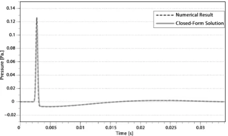
Interpolated Wideband(IWB) scheme, with the free parameters set toa= 1/4,b= 1/16andX = 28.62mm. The transient sound pressure, obtained at the receiving position0.5m away from the source in the axial direction, is shown in figure 3. For comparison purposes, the sound pressure at the receiving position was also calculated in closed form using equation (12), and is shown as reference (solid line) in figure 3.

Figure 3:Sound pressure response at the receiving position. Nu-merical results (dashed line) are compared to the closed-form so-lution(12)to the wave equation (solid line).

frequen-cies the discrepancy increases, which is particularly visible for the largest value ofη. This is attributed to the fact that whilst the an-alytic solution assumes spherical symmetry, the dispersive proper-ties of the FDTD method cause anisotropy that grows stronger as frequency is increased. The choice ofηis therefore a compromise between bandwidth and the amount of dispersion introduced by high frequencies.

Figure 4:Frequency response of the sound pressure at the receiv-ing position. Numerical results (dashed lines) are compared to closed-form solutions(12)to the wave equation (solid lines).

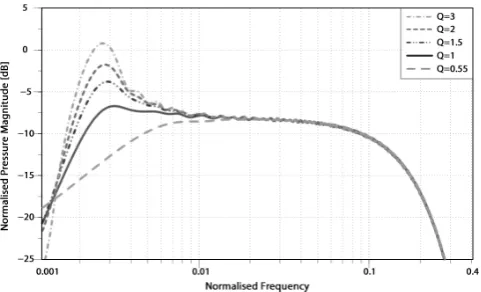
The effects ofQon the low frequency behaviour of the system are shown in figure 5. As expected, the higherQis, the more pro-nounced is the low-frequency resonance of the system. It can be

Figure 5:Frequency response at the receiving position withQ= 0.55(heavy dashed),Q = 1(solid), Q = 1.5(triple dashed),

Q= 2(dashed) andQ= 3(double dashed). The high cut-off is setη= 0.75for all curves.

seen that the flatness of the response at low frequencies is strongly affected by the choice ofQ, in a similar fashion to a real-world transducer. AtQ = 0.55, when the system is nearly critically damped, the magnitude response rolls off as a near straight line. MakingQhigher allows extending the low frequency bandwidth at the expense of a more pronounced resonance and a more abrupt transition. This is the type of compromise that a loudspeaker de-signer faces when choosing a driver and enclosure. In such cases, the totalQof the electro-mechanical system typically ranges be-tween0.5and2.0[10].

4.2. Numerical Consistency

An important feature of the PCS model is that it yields consistent results across different sample rates. Since the source function is correctly scaled with FDTD grid parameters (see equation 9), then for a given volume velocity the resulting pressure is independent of sample rate. Clearly, if the source areaAsis chosen such that it varies with the spatial sample period, then so will the correspond-ing volume velocity and the resultcorrespond-ing pressure at the source posi-tion. Thus, if one wishes to preserve numerical consistency, then Asshould be held constant even if the sample rate is changed.

To test this, two simulations were carried out at grid resolu-tions ofX = 19mm andX= 10.7mm. Since the total source en-ergy depends on the variance of the Gaussian driving force which normally depends onfsas well asη, here a constantσwas main-tained in order to ensure that an identical amount of energy was injected into the grid at both resolutions. Simulations were re-peated for three types of sources. First, we examine the typical

hard sourcemethod in which the driving function,ψ(t), is directly imposed on the source grid node, i.e

p

n+1

l0,m0,i0=ψ

n+1

(31)

where in this caseψis simply considered to be a Gaussian func-tion. Next, we test asoft sourcederived from a 1D waveguide analysis as presented in [8], withqˆ(t)being differentiated, scaled and superimposed on the source node, such that:

p

n+1

l0_,m0_,i0= n

p

n+1

l0_,m0_,i0 o

+ψ

n+1

(32)

whereψ

n+1

= ρ0c 2X

ˆ

q

n+1

−qˆ

n−1

, andqˆis considered to be a volume velocity with a Gaussian distribution to which the phys-ical model presented herein hasnotbeen applied. Lastly, we con-sider thephysically-constrained sourcemodel withAskept con-stant across the two different grid resolutions.

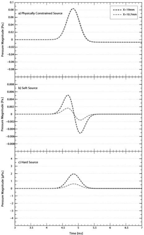
It can be seen from figure 6 that whilst the hard and soft sources exhibit different pressure magnitudes at the receiving position, the amplitude of the physically-constrained source remains identical at different grid resolutions. It should be noted, however, that for a one-dimensional waveguide, one would expect a similar behaviour from a soft source given that it has been appropriately scaled as shown in [8].

4.3. Frequency Response

The frequency response curves of the three different source models described in 4.2 are shown in figure 7. Here, the pulsating sphere system was designed with its natural resonance at the normalised frequencyf0T = 0.002, andQ= 1. It can be seen that the

fre-quency response of the PCS is nearly as flat as the hard source. The soft source exhibits the frequency response of a differentiated Gaussian, as it lacks the mechanical filter included in the PCS for-mulation.

4.4. DC Effects

Figure 6: Impulse responses generated at grid resolutions of

X= 19mm (dark curves) andX= 10.7mm (light curves), for a) Physically constrained source, b) Soft Source and c) Hard Source. Simulations performed withf0= 30Hz,M = 25g andQ= 1.25.

The force driving function is a Gaussian pulse which is identical in shape to panel (c). A more detailed evaluation of the driving function is shown in Figure 2.

of arbitrary amplitudeA, interacting with a surface having a re-flection coefficientˆr, the total sound pressure along the plane is p(x, t) =Aej(ωt−kx)_{+ ˆrAe}j(ωt+kx)_{. As such, the sound}

pres-sure at DC is uniformlyp=A(1+ˆr)along the plane. Since source injection is additive, then for anyˆr >0a pre-existing DC com-ponent would constructively superimpose on itself at the source node, resulting in an incremental offset.

To exemplify this, consider an additive source injection as shown in equation (32), driven directly by a Gaussian excitation function, such that

ψ(t) =Ae−(t

−t0)2

2σ2 ₍₃₃₎

Being a unipolar function, the Gaussian source exhibits a strong DC component, thus we expect solution growth. Unlike the soft

Figure 7: Frequency response of three types of sources: Hard Source (HS, heavy dashed), Soft Source after Karjalainen and Erkut [8] (SS, triple dashed-dotted) and Physically-Constrained Source as presented in this paper (PCS, regular dashed). All sources were generated withη= 0.75, and the PCS was designed with a normalised resonance atf0T = 0.002andQ= 1.

source described in section 4.2, this function does not get differ-entiated prior to being injected in additive form, and as such, will be further referred to as anArbitrary Soft Source. As reference, consider the same excitation function, however being filtered and injected according to the PCS principles, which is summarised in Figure 1. As will be further discussed, the PCS model acts as a nat-ural DC-blocking filter, therefore no solution growth is expected. The result of this comparison is shown in Figure 8.

Figure 8:Sound pressure response at the receiving position, due to an arbitrary soft source (SS - dark solid line) plotted against a physically constrained source (PCS - light solid line). Note that the magnitude scale of the soft source is different. Both simulations where executed with uniform boundary conditions corresponding torˆ= 0.997.

Such behaviour is also sensible from a physical perspective, as a DC component inψ(t)indicates thatq(t)is not of finite length, meaning that the source endlessly generates volume velocity. Fol-lowing equation (11), the rate of fluid emergence due to the arbi-trary soft source is obtained by taking the integral of equation (33) which yields

q(t) =

Z

ψ(t)dt=

r

π

2AσERF

t−t0

√

2σ

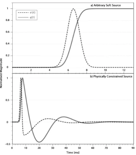
whereERF(·)is the Gauss error function. Figure 9 shows the com-parison of an additive functionψ(t)plotted against its correspond-ing rate of fluid emergenceq(t), for an arbitrary soft source (after equations (33) and (34)) and a physically constrained source. Sim-ilar effects have been observed in the field of computational elec-trodynamics [11]

Figure 9: Comparison ofψ(t)andq(t) for two source models, a) arbitrary soft source directly driven by a Gaussian function; and b) physically-constrained source driven by a Gaussian force. Results have been normalised for visual clarity.

For the PCS, bothq(t)andψ(t)start at zero and decay to zero, indicating a finite source. However, this is not the case for the ar-bitrary soft source. The fact thatψ(t)seems time-limited can be misleading, as it only physically means that the source generating mechanism does not accelerate before or after the excitation pe-riod. This, of course, does not mean that the source is not active. In fact, it can be seen that whenψ(t)decays,q(t)rises and stays at a constant value through the remaining simulation period. This in-dicates that even whenψ(t)is time limited, the source mechanism may still generate volume velocity. As one would expect,q(t) re-mains at a constant positive value which is equivalent to generation of DC.

5. DISCUSSION

The PCS model described in this paper provides means to design sources of prescribed pressure. In a free field, results show very good matching with the closed-form solution to the wave equa-tion, which underlines the physical basis of the approach. Dis-crepancies are mostly attributed to the numerical artefacts of the system, which include spatial quantisation and dispersion. Both of these can be greatly reduced by means of oversampling, choos-ing an appropriate numerical scheme, and/or spatial interpolation.

To demonstrate the benefits of the PCS model, we have used a Gaussian pulse as a driving force. The source signal is truncated at points chosen such that the resulting discontinuity errors largely fall below the numerical errors due to the finite difference approx-imations. Consequently, such an excitation function is a suitable candidate for the requirements of an FDTD source, as it is both band-limitedandsufficiently time-limited. The model is also ap-plicable to other excitation signals.

The importance of scaling and differentiating additive sources has been clearly identified in this work. Correct magnitude scal-ing of the excitation signal is essential for obtainscal-ing consistent re-sults when numerical parameters are altered. More importantly, the magnitude scaling of the PCS model yields results that con-verge well with the analytic solution, which is not the case for other sources. The model inherently handles differentiation of the source function, which eliminates the DC component from the source term, thus avoiding any undesirable signal growth. Follow-ing equation (11), the source function in the frequency domain isΨ(ω) = jωQ(ω), which is null forω = 0. This requires thatq(x, t)is differentiable in time and thatq(x,±∞) = 0. The former can be satisfied by choosing a sufficiently smooth driving function. The latter criterion requires that the pulsating sphere be-gins at its resting position and returns to that position after the excitation period. Close observation of equation (4) shows that

lim

t→∞M e −αt

= 0 , ∀α >0 (35)

therefore ifF(t)begins and ends at zero, andαis positive, then bothq(t) and ψ(t) are appropriately time-limited, as has been shown to be the case in section 4.4. A suitableF(t)can be ob-tained by employing an adequately finite function witht0 > 0. A positiveαsimply means that the mechanical system must be damped. This affirms that the pulsating sphere model acts as a natural DC blocking filter.

Similar issues concerning scaling and differentiation have been briefly discussed in [8]. However, being drawn from 1D digi-tal waveguide theory, the proposed scaling is inadequate for 3D schemes. Furthermore, an appropriate excitation signal is not plicitly defined. It has been shown that employing an arbitrary ex-citation signal in additive form can result in solution growth (see figure 8), or if it has been differentiated then the observed pres-sure signal is high-pass filtered (see figure 7). In the PCS model, the mass reactance of the sphere acts as an integrator which, in a physical manner, counters the effects of differentiation. Be-low its resonant frequency, the system is stiffness dominated, and as such, naturally acts as a DC-blocking filter. The result is a source having a near-flat pressure spectrum (see Figure 4) whose physical properties can be freely chosen by adjustingQandω0.

Thus, the PCS model adheres to physical laws but is not lim-ited by real-world engineering constraints. Technically, it is pos-sible to empirically design a source function which is compati-ble with an arbitrary soft-source injection by passing the excita-tion signal through a simple DC-blocker with the transfer funcexcita-tion H(z) = (1−z−1)/(1−az−1). For differentiated soft-sources, one may also consider using the first time integral of any function which does not have a DC component. Yet, the PCS method offers a more structured and physically-oriented approach for achieving these goals.

scattering incoming waves, thus as far as frequency response is concerned, they offer a good alternative to the PCS method. How-ever, the PCS method also physically relates the excitation func-tion to grid parameters, and as such, is the only method which is numerically consistent by default. Furthermore, transparent sources are more computationally expensive, and are prone to the same low frequency artefacts as hard sources [5], which is not the case of the PCS.

6. CONCLUSION

In the numerical domain, the source model described in this pa-per can be thought of as adiscrete point-monopolewhich is con-strained by physical laws. Two systems govern the source, the first being the mechanical pulsation of a small sphere, and the second being the transduction of motion into acoustic pressure. To the authors’ knowledge, this is the first time where these two systems have been integrated into a single physically-plausible model, at least in context of FDTD simulation. This approach offers vari-ous benefits over existing source models. It provides means to de-sign and inject sources which generate a prescribed pressure field, do not scatter incoming waves, and have a near-flat frequency re-sponse without causing any low-frequency artefacts. Furthermore, the method is correctly scaled with FDTD parameters, and thus is numerically consistent across different sample rates. The two systems governing the source are uncoupled, which is a reason-able assumption as the pulsating sphere is considered to be very small. A more realistic model would consider numerical coupling of the two systems, which remains an interesting topic for future research.

7. ACKNOWLEDGMENTS

The authors would like to thank Mark Avis for insightful discus-sions on sound generating mechanisms, and three anonymous re-viewers for their valuable comments and suggestions.

8. REFERENCES

[1] K. Kowalczyk and M. van Walstijn, “Room acoustics sim-ulation using 3-D compact explicit FDTD schemes,” IEEE Transactions on Audio, Speech, and Language Processing, vol. 19, no. 1, pp. 34–46, 2011.

[2] S. Bilbao, “Optimized FDTD schemes for 3D acoustic wave propagation,” IEEE Transactions on Audio, Speech, and Language Processing, , no. 99, pp. 1–1, 2012.

[3] L. Savioja, “Real-time 3D finite-difference time-domain simulation of low-and mid-frequency room acoustics,” in

13th Int. Conf on Digital Audio Effects, 2010.

[4] F. Fontana and D. Rocchesso, “Physical modeling of mem-branes for percussion instruments,” Acta Acustica united with Acustica, vol. 84, no. 3, pp. 529–542, 1998.

[5] H. Jeong and Y.W. Lam, “Source implementation to elimi-nate low-frequency artifacts in finite difference time domain room acoustic simulation,”Journal of the Acoustical Society of America, vol. 131, no. 1, pp. 258, 2012.

[6] J.B. Schneider, C.L. Wagner, and S.L. Broschat, “Imple-mentation of transparent sources embedded in acoustic finite-difference time-domain grids,”The Journal of the Acoustical Society of America, vol. 103, pp. 136, 1998.

[7] D. Botteldooren, “Finite-difference time-domain simulation of low-frequency room acoustic problems,” The Journal of the Acoustical Society of America, vol. 98, pp. 3302, 1995. [8] M. Karjalainen and C. Erkut, “Digital waveguides versus

fi-nite difference structures: Equivalence and mixed modeling,”

EURASIP Journal on Applied Signal Processing, vol. 2004, pp. 978–989, 2004.

[9] P.M.C. Morse and K.U. Ingard, Theoretical acoustics, Princeton Univ Pr, 1986.

[10] R. H. Small, “Closed-box loudspeaker systems-part 1: Anal-ysis,” J. Audio Eng. Soc, vol. 20, no. 10, pp. 798–808, 1972. [11] T. Su, W. Yu, and R. Mittra, “A new look at FDTD excitation sources,” Microwave and optical technology letters, vol. 45, no. 3, pp. 203–207, 2005.

9. APPENDIX I: UPDATE EQUATION FOR AIR

The update equation for air,

n

p

n+1

l0_,m0_,i0 o

, is required in order to evaluate the source node in an additive form. Readers who wish to implement the compact explicit schemes discussed in section 3.1 may use the following air update equation:

p

n+1

l,m,i=d4p

n l,m,i−p

n−1

l,m,i+d1

X

p

a

| {z }

axial

+d2 X

p

sd

| {z }

side-diagonal

+d3 X

p

d

| {z }

diagonal

whereP

p

a,

P

p

sdand

P

p

dare the sums of pressures of the neighbouring nodes at the axial, side-diagonal and diagonal direc-tions, respectively. The coefficientsd1,d2,d3andd4 are

calcu-lated from the free parametersaandb, and are given by

d1 = λ2(1−4a+ 4b)

d2 = λ2(a−2b)

d3 = λ2b

d4 = 2 +λ2(12a−8b−6)