Modelling and simulation for the joint maintenance inventory optimisation of production systems

Modelling and simulation for the joint 

maintenance­inventory optimisation of 

production systems

Zahedi­Hosseini, F

http://dx.doi.org/10.1109/WSC.2018.8632283

Title

Modelling and simulation for the joint maintenance­inventory optimisation 

of production systems

Authors

Zahedi­Hosseini, F

Type

Conference or Workshop Item

URL

This version is available at: http://usir.salford.ac.uk/48235/

Published Date

2019

USIR is a digital collection of the research output of the University of Salford. Where copyright 

permits, full text material held in the repository is made freely available online and can be read, 

downloaded and copied for non­commercial private study or research purposes. Please check the 

manuscript for any further copyright restrictions.

M. Rabe, A.A. Juan, N. Mustafee, A. Skoogh, S. Jain, and B. Johansson, eds.

MODELLING AND SIMULATION FOR THE JOINT MAINTENANCE-INVENTORY OPTIMISATION OF PRODUCTION SYSTEMS

Farhad Zahedi-Hosseini University of Salford

Manchester

M5 4WT, UNITED KINGDOM.

The text in yellow has either been added or highlighted in response to comments from Reviewer 1. The text in pink has either been added or highlighted in response to comments from Reviewer 2.

ABSTRACT

Simulation methodologies are developed to model the joint optimization of preventive maintenance and spare parts inventory for a specific industrial plant under different production configurations. First, spare parts provisioning for a single-line system is considered, with the assumption that the demand is driven by maintenance requirements. The results indicate that a periodic review policy with replenishment as frequent as inspection is cost-optimal. Second, the joint optimization model for a multi-line (parallel) system is developed. It is found that a just-in-time review policy with inspection as frequent as replenishment produces the lowest cost policy. In this latter case, an implication of the proposed methodology is that, where mathematical modelling is intractable, or the use of certain assumptions make them impractical, simulation modelling is an appropriate solution tool. Under both production settings, the long-run average cost per unit time is used as the optimality criterion for the comparison of several policies.

1 INTRODUCTION

For several decades, many journal papers have been published that demonstrate an intense research in using maintenance analysis in the area of Production and Operations Management (Wang 2012). In particular, scholars have shown an ever-growing interest in the analysis of plant downtime and the management of its associated spare parts inventory. Minimizing maintenance costs or system downtime, or maximizing system availability, may be some examples of the focus in the objective function for the primary purpose of maintenance optimization.

Many review papers have appeared in the maintenance literature including the most recent publications by: Pophaley and Vyas (2010); Das and Sarmah (2010); and Van Herenbeek (2013). Analytical models that are discussed in these reviews are based on simple assumptions. To relax or eliminate some assumptions of these models might make them unsuitable to be implemented in practice. As an appeal to maintenance modelers, Scarf (1997) states: “too much attention is paid to the invention of new models, with little thought, it seems, as to their applicability”. The same observation still seems valid since “little research is conducted on the optimization of maintenance in industrial systems” (Alrabghi et al. 2017).

The rest of this paper is organized as follows. Sections 2 and 3, review the maintenance and inventory control policies. Section 4, describes the simulation tool used. Sections 5 and 6, give details of the modelling for two case examples: a single machine, and a parallel production facility, respectively. The final section summarizes conclusions for the case examples, and highlights the future direction of our research.

2 MAINTENANCE POLICIES

Van Horenbeek et al. (2013) give detailed account of the three main maintenance strategies: (i) corrective; (ii) preventive; and (iii) predictive maintenance.

Under the corrective maintenance, whenever a unit fails, it is immediately repaired or replaced by a new one, provided spares are available. Consequently, if no spare is available, equipment downtime will occur and the system will have to await the delivery of emergency parts while they are in transit.

Equipment may also be maintained under a preventive strategy, where failed units are replaced too, but all other units are also ‘block-replaced’ at constant intervals regardless of their history, current condition, and age. This is the periodic block-based strategy. In comparison, if the machine or equipment lends itself to being maintained based on the age of the unit, then the well-known age-based preventive maintenance, first suggested by Barlow and Hunter (1960), may be used. Under this policy, apart from the units that have failed in service, the rest are replaced whenever they reach their predefined age. Finally, under an inspection-based preventive strategy, failed parts are replaced immediately, and faulty parts are replaced at regular inspection intervals (for example, Wang 2008). Evidently, there is a strong link between the inspection interval and the replacement part inventory. If the inspection interval is too short, then the ‘lumpy’ demand effect is created. This is the result of replacing multiple defective but still working parts to reduce the risk of failure at a later stage. Equally, if the inspection interval is too long, then the number of single-unit parts randomly failing is increased, adding to downtime.

Finally, under the predictive maintenance strategy (better known as condition-based maintenance, CBM), the state of the system is continuously observed and monitored. And, where certain or a combination of ‘signals’, such as, vibration or heat, for example, reach a prescribed limit, maintenance action is undertaken and units may be replaced (see, Olde Keizer et al. 2017 for the latest review paper).

Whichever maintenance strategy is used to restore the system under consideration, different costs will be incurred. These costs could include, for example, inspection, downtime, labor and spare replacements. A distinction must also be made between failure replacement and preventive replacement, which will have a different cost element for the associated labor and downtime costs.

In this paper, we use an inspection-based maintenance strategy. Five factors would influence the determination of the optimum inspection interval and thus minimizing the cost of downtime. First, the timing and the rate of arrival of defects. Second, the time it takes defects to cause failures. Third, the pace at which inspections are undertaken. Fourth, the cost and downtime associated with inspections and defect removal (by replacing/repairing parts). Finally, the cost and downtime associated with replacing/repairing failures. Thus, using a modelling tool for determining the optimal period for 𝑇 would be beneficial in guiding the decision-making process.

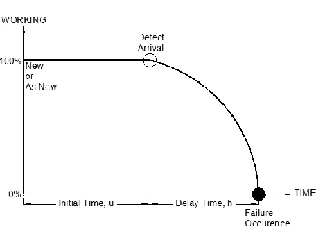
Figure 1. The delay-time concept.

Delay-time modelling captures the relationship between failures of items in service, inspection at constant PM epochs, and PM replacement of defective items under the assumption that all defective items are always identified and replaced (provided spares are available) at inspections. Since its conception in 1976, a few detailed review papers have been published on delay-time modelling, the latest by Wang (2012). There are also many delay-time-based case study applications reported in the literature including recently by Emovon et al. (2016).

3 INVENTORY CONTROL POLICIES

Maintenance costs are clearly dependent on the availability of spare parts. However, many models assume there is an infinite inventory of spare parts at all times, which makes their use unrealistic in practice. The inventory for spare parts is normally controlled by a particular replenishment policy. The overall objective is always to find the optimal policy. Keeping too many spares will increase the holding cost, which will have financial implications on the company’s cash flow and/or borrowing, or will increase the risk of spare parts’ obsolescence. Conversely, keeping too few parts might result in the plant’s unavailability at critical times. The cost associated with the unavailability of spare parts include the cost of equipment downtime while awaiting spare delivery, and the cost of expediting the delivery of parts in emergencies.

There are two distinct approaches of ‘periodic’ or ‘continuous’ replenishment for the management of spare parts (see, for example, Muller 2011). Under the periodic review policy, there are at least three methods by which parts may be replenished. First, the (𝑅, 𝑆) policy - periodically(𝑅), at the beginning of each cycle, raising the inventory position to a pre-defined level, 𝑆. Second, the (𝑅, 𝑠, 𝑆) policy - periodically raising the inventory position to level 𝑆 if the stock level has reached or dropped below a certain level, 𝑠. Finally, the (𝑅, 𝑠, 𝑄) policy - periodically raising the inventory position by ordering a fixed quantity 𝑄 of stock if the inventory position has reached or dropped below 𝑠 (see, for example, Silver et al. 2016).

parts increases the cost of inventory and the risk of obsolescence, which is a major issue and has cost implications too.

4 MODELLING TOOL

Simulation has been used for many years to understand and experiment with systems under study, especially in the production and manufacturing industry, where the use of discrete-event simulation (DES) has been very effective. The use of simulation has grown dramatically since modern manufacturing systems have become more complex due to dependencies and interactions between system components. Gupta and Lawsirirat (2006) highlight the fact that the term component has a different meaning in different contexts. Since it is not possible to model every part in a complex system, it is practical to consider only the components that have significant impact on the performance of the system.

Simulation delivers an advantage over analytical approaches since many maintenance policies are not analytically traceable (Nicolai & Dekker 2008). Mathematical approaches are limited in solving such complex maintenance problems.

A very important step forward in the world of simulation is the obvious and essential procedures for verification and validation, which can only lead to credibility of simulation models and the results achieved from them (Rabe and Dross 2015). The gap between research in optimization via simulation and the development of algorithms that can be applied to real-life problems has narrowed substantially in the last ten years. One factor influencing this issue is the ever-growing use of parallel simulation, which is becoming easy to do, and any simulation study that requires multiple replications or multiple scenarios will benefit from this advancement (Nelson 2016).

For developing the simulation models in this paper, ProModel (ProModel 2016), a process-based discrete-event simulation language, (see for example, Harrell et al. 2011), one of many proprietary simulation packages available in the market, was used. The models were developed as continuous production lines. To ensure that the optimal cost is achieved, SimRunner (see ProModel 2010), a simulation optimization tool, was integrated with the simulation models, which performs sophisticated analysis to determine the optimal value of decision variable(s). The optimization tool automatically runs multiple combinations of certain variables (if needed) to find the unique combination, which provides the optimal value of the objective function ~ the long-run average expected cost. When optimizing a particular system, one might use exact solution methods (analytical), or heuristic methods to find near optimal values for the decision variables. Safety factors, various service levels, system downtime, or costs, are a few examples, which may be used as a focus in an optimization study. The minimization of the costs is most common in the optimization of maintenance-inventory problems (Van Horenbeek et al. 2010), which is also used for the models in this paper.

5 CASE EXAMPLE 1

In case example 1, we consider a specific industrial plant situation. In particular, we develop simulation models for jointly optimizing the inspection maintenance for a paper mill, and the inventory policy for bearings, which are critical components in the plant. Paper machinery typically have many identical bearings, and their failure or lack of proper maintenance can incur various costs (Folger et al. 2014), such as, improper handling and installation; inadequate lubrication; contamination; and various overload. The consequences of damage to a bearing system in industrial machinery can be very significant in terms of general risk to safety and financial implications including machine downtime, and cost of replacement. Therefore, it is appropriate to develop models for reducing the risk of failure and system downtime.

We assume that the plant has n identical bearings (Wang 2011), which are subject to deterioration. Multiple concurrent defects are possible in the plant and the failure process of a bearing has two-stages, according to the delay-time concept described in Section 2 (Figure 1), and further illustrated in Figure 2.

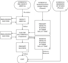
Figure 2. Defect arrivals and failure occurrences in our complex system of multiple components. External specialists (Wang and Wang 2015) inspect all bearings, in parallel, every T time units, and defective bearings are replaced preventively, as depicted in Figure 3. The ‘Failure Occurrence’ in Figure 3 denotes that whether it is a planned (intervention) or unplanned event, it will result in machine downtime. On failure, failed bearings are replaced immediately if spare parts are available, when inspection of other bearings does not take place. We assume the system is in a state of suspension whilst the plant is not operating. Therefore, defects do not grow and the bearings do not age during replacement downtime. Any other operational activity other than inspection, replacement and failure are ignored (Wang 2011, 2012).

PROLONGING ROUTINE 5 PROLONGING ROUTINE 5 DEFECT ARRIVAL 2 FAILURE OCCURRENCE (Unplanned) 3 PREEMPT MACHINE 4 PREEMPT DEFECTS WAITING IN THEIR ‘DELAY TIME’ 7 REMOVE DEFECTS WAITING IN THEIR ‘DELAY TIME’ 8 SCHEDULE PRE-DEFECT ARRIVAL 1 SCHEDULE MAINTENANCE INSPECTIONS (Planned) 6 EXIT Pre-defect Defect Defect(s) Failure Defect(s) Removed SCHEDULE ORDERING OF SPARES (Planned) 9

Figure 3. Flowchart of the general simulation procedure.

Defect arrivals are assumed to be independent and exponentially distributed, while the delay-time has a Weibull distribution. The individual machine downtime cost-rate = £1,000 per hour. This information and others in the model are based on our consultation with paper-making manufacturers.

The demand for bearings is generated through two routes: (i) failures of parts in service between inspections; and (ii) at scheduled inspections, every T time units, provided there are enough spares.

T Defect arrival Failure

Otherwise, demand will be satisfied by expediting an emergency order. We assume that the system is operating under steady-state conditions.

We will compare several periodic review inventory policies (see, for example, Silver et al. 2016). As depicted in Figure 4, these policies include the (𝑅, 𝑆), the (𝑅, 𝑠, 𝑆), and finally, the (𝑅, 𝑠, 𝑄). For all three policies illustrated in Figure 4, with the same arbitrary demand profile, orders are placed at points A, C, and E, for example, and arrive at points B, D, and F respectively, after a lead-time, 𝐿.

We set the normal delivery cost at £100; the cost-rate of inventory holding, at 1% of item cost per week; and finally the emergency shipment cost, set to £1,000 per emergency order. In all three cases, the joint policy contains the decision variable T, the inspection interval. However, other decision variables depend on the choice of the periodic review inventory policy. In the model, we are interested in values of the decision variables that minimize the long run expected cost per unit time (cost-rate).

Figure 4. Inventory positions of the periodic review inventory policies.

Three joint inventory-maintenance policies were considered: (𝑅, 𝑆, 𝑇 = 𝑅), (𝑅, 𝑠, 𝑆, 𝑇 = 𝑅), and

(𝑅, 𝑠, 𝑄, 𝑇 = 𝑅). Table 1 illustrate that the (𝑅, 𝑆, 𝑇 = 𝑅) policy has the lowest cost-rate (total cost per unit time), inspecting the bearings in the plant and ordering spares every 9 weeks. Note that, the (𝑅, 𝑠, 𝑆, 𝑇 = 𝑅) policy is equivalent to the cost-minimal policy because 𝑆∗− 𝑠∗= 1, where 𝑆∗and 𝑠∗ are the optimum values of 𝑆 and 𝑠 respectively.

Table 1. Cost-rate comparison. Lowest cost-rate for each policy. Overall cost-optimal policy(s). (R,S,T=R) (R,s,S,T=R) (R,s,Q,T=R)

T Cost* S Cost* s S Cost* s Q

5 698.07 3 698.07 2 3 704.70 2 2 6 660.35 3 660.35 2 3 664.08 2 2 7 640.27 3 640.27 2 3 644.57 2 2 8 624.79 3 624.79 2 3 624.12 2 2 9 611.81 3 611.81 2 3 612.00 2 2 10 612.64 4 612.64 2 3 612.48 2 2 11 614.21 4 614.21 2 3 616.04 2 2 12 616.87 4 616.87 2 3 620.06 2 2 13 622.11 4 622.11 2 3 627.82 2 2 14 627.84 4 627.84 2 3 635.90 2 2 15 633.85 4 633.85 2 3 638.71 2 2

R R

0 S

s

Inve

ntory Level

L L L

R R R

S

L L

R R R

L

0 0

s

Time

R, S policy R, s, S policy R, s, Q policy

A B C D E F A B C D E A B E

T1 T2 T3 T1 T2 T3 T1 T2 T3

L C D Q

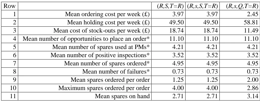
Table 2, row 1, illustrates that the (𝑅, 𝑆, 𝑇 = 𝑅) policy (similar to (𝑅, 𝑠, 𝑆, 𝑇 = 𝑅)) has a higher ordering cost-rate than the (𝑅, 𝑠, 𝑄, 𝑇 = 𝑅) policy since it can potentially place more orders at both inspections and at failures. This is also partly because 𝑠 = 2 and 𝑆 = 3, whence an order is always triggered when the stock level drops by one unit, compared to the (𝑅, 𝑠, 𝑄, 𝑇 = 𝑅) policy, where twice as many stock is ordered every time (since 𝑄 = 2). So, the latter policy must have a lower order cost-rate since it places fewer orders, but higher quantities every time. This observation is supported by row 9 since the mean number of spares ordered per order is higher for the (𝑅, 𝑠, 𝑄, 𝑇 = 𝑅) policy.

Similar observations to those made about order cost-rates can be made about holding and stock-out cost-rates, displayed in rows 2 and 3, respectively. The (𝑅, 𝑠, 𝑄, 𝑇 = 𝑅) policy has a higher holding and a lower stock-out cost-rates since it orders twice as many stock every time. Therefore, inventory costs seem to be traded off: where the holding cost-rate is high, the stock-out cost-rate is low, and vice versa.

Table 2. For the optimum policy in each class of inventory policies (*per 100 weeks).

Row (R,S,T=R) (R,s,S,T=R) (R,s,Q,T=R)

1 Mean ordering cost per week (£) 3.97 3.97 2.45 2 Mean holding cost per week (£) 49.50 49.50 58.81 3 Mean cost of stock-outs per week (£) 18.74 18.74 11.49 4 Mean number of opportunities to place an order* 11.10 11.10 11.10 5 Mean number of spares used at PMs* 4.21 4.21 4.21 6 Mean number of positive inspections* 3.52 3.52 3.52 7 Mean number of spares ordered* 4.95 4.95 4.95 8 Mean number of failures* 0.73 0.73 0.73 9 Mean spares ordered per order 1.25 1.25 2.00 10 Maximum spares ordered per order 4.00 4.00 2.86 11 Mean spares on hand 2.71 2.71 3.14

Rows 4 to 8, as expected, that the average values for the following data are similar for all three policies: the number of opportunities to place an order; usage rate of spares at PMs; number of positive inspections (i.e. one or more defects found); number of spares ordered; and finally, number of failures, respectively. So, the consumption of parts (at steady state) must be most influenced by the rate of arrival of defects, which is the same for all three policies in our model.

6 CASE EXAMPLE 2

The specific industrial situation considered in this second case example is also a paper mill, but this time, consisting of two machines working in parallel. As before, beside relatively low-cost cutting blades, bearings are the critical components in this plant.

is subject to preventive replacement or failure replacement, then simultaneous downtime cost is incurred. Preventive replacement cost is not affected in this way because a preventive replacement waits until a failure replacement is complete. Note, it is this kind of complexity that makes the use of simulation very useful and effective, and may be very difficult or impossible to obtain using analytical modelling.

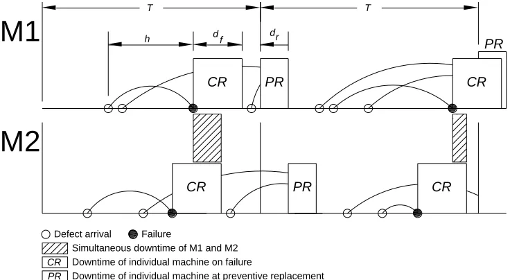
Figure 5. Two machines, M1 and M2, inspected periodically at interval 𝑇, in parallel, downtime 𝑑𝑟 due to

preventive replacement, and downtime 𝑑𝑓due to corrective replacement (𝑑𝑟 < 𝑑𝑓).

The individual machine downtime cost-rate = £1,000 per hour, and the simultaneous machine downtime cost-rate = £10,000 per hour since it halts production. As before, these parameter values were set in discussion with manufacturers, which ensured that our model and simulation experiments are realistic and not based on some arbitrary data.

We consider the (𝑅, 𝑆) replenishment policy since, in case example 1, it was demonstrated as the best policy amongst other periodic review replenishment policies. Therefore, stock is reviewed every 𝑅 time units and an order is placed to bring the inventory position up to level 𝑆, if needed.

Two joint inventory-inspection policy variants are considered: (𝑅, 𝑆, 𝑇 = 𝑅), with coincident and just-in-time ordering. Under the former policy, inspection and review of the inventory position coincide. In the later variant, the inventory position is reviewed ‘lead-time’ units before the next inspection, so that stock (if ordered) arrives just in time for the next inspection. For both variants, there are three decision variables: the review period, 𝑅; the inspection interval, 𝑇; and the order-up-to level, 𝑆. We sought those values of the decision variables that minimize the long-run total cost per unit time (cost-rate).

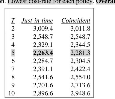
Table 3 shows the results for the two policy variants. It illustrates that the (𝑅, 𝑆, 𝑇 = 𝑅) policy using

just-in-time ordering has the lowest cost-rate, inspecting bearings every 5 weeks, reviewing stock at the same frequency and ordering sufficient spares to return the inventory position to the optimum. It is important to note that, although scheduled inspection times are known, the times of demands for spare parts are unknown. Consequently, in order to eliminate, or at least minimize, the occurrence of simultaneous downtime, it is important to consider, relative to inspection, when and in what quantity spares are ordered.

T T

d

d _r

f

PR

CR CR

PR

h

PR

CR CR

Defect arrival Failure

Simultaneous downtime of M1 and M2

M1

M2

Downtime of individual machine on failure

Downtime of individual machine at preventive replacement

Table 3. Cost-rate comparison. Lowest cost-rate for each policy. Overall cost-optimal policy.

T Just-in-time

Coincident

2 3,009.4 3,011.8 3 2,548.7 2,548.7 4 2,329.1 2,344.5

5 2,263.4 2,281.3

6 2,284.7 2,304.5 7 2,391.1 2,422.4 8 2,541.6 2,554.0 9 2,701.6 2,713.6 10 2,896.6 2,948.6

Comparing the ordering cost-rates for the two policies, Table 4 demonstrates, as expected, that the costs are the same. The holding cost-rate appears to have a significant effect on the choice of policy since it is mainly influenced by the frequency of review and the order-up-to level 𝑆. Clearly, the timely review of the stock, ordering (just-in-time) up to the optimal level 𝑆, will result in keeping less stock and a lower holding cost-rate. Whereas the difference between the best cost-rates of the two policies is only £17.90 (0.8%, as shown in Table 3), the difference between the holding cost-rates for the same inspection interval is £5.68 (as shown in Table 4), which accounts for 32% of the cost difference. This implies that the holding cost-rate has a significant effect on the choice of policy.

Table 4. For the optimum policy in each class of inventory policies.

Row JIT Coincident

1 Mean ordering cost per week (£) 14.28 14.28 2 Mean holding cost per week (£) 14.26 19.94 3 Mean cost of stock-outs per week (£) 5.42 0.68 4 Mean simultaneous machine downtime cost per week (£) 8.02 8.73

Although, the simultaneous machine downtime cost does not seem to be a significant contributor to cost-rate; however it aligns with the policy ranking. Both holding cost-rate and simultaneous machine downtime cost-rate display a similar pattern. It is interesting to note that, the (𝑅, 𝑆, 𝑇 = 𝑅) policy using

coincident ordering, may be perceived as a low risk policy since it has a low stock-out cost-rate. Obviously, the just-in-time ordering must have the greatest influence on the choice of policy. In addition, component cost-rates are traded-off which place different demands on inventory.

7 CONCLUSIONS

In this paper, we have developed several simulation models for the joint maintenance-inventory optimization of a paper mill under two different manufacturing configurations. Without the use of modelling, it will be unclear when inspections should be performed, when spares should be ordered and in what quantity, since parameter values will be random. In both case example simulations, a warm-up period of 1,000 weeks, and 10,000 weeks of simulation run with three replications deemed appropriate.

order spares every 9 weeks (the review period) to raise the inventory position to level S (using the

(𝑅, 𝑆) policy). More frequent inspection, and hence ordering, increases planned costs and in compensation decreases unplanned costs due to bearing failure and machine downtime.

Second, simulation models were developed to study the maintenance and spare parts inventory of a paper mill facility with two machines, working in parallel. We assume that simultaneous machine downtime stops production completely, which incurs significant cost. The (𝑅, 𝑆, 𝑇 = 𝑅) just-in-time policy, inspecting, reviewing, and ordering stock (if needed) at the same frequency is cost-optimal. Ordering in advance of inspection reduces holding costs since, on average, less stock is held. We deliberately used the same (𝑅, 𝑆) policy, which proved to be the cost-optimal policy in our first case example. For the optimum policy, the sensitivity analysis to different parameters gives results that are broadly expected. The defect arrival rate and the cost of emergency shipment parameters have the most and least impact, respectively.

Joint maintenance-inventory models, and specially models of parallel systems, require complex mathematical formulations, which may not be possible to solve analytically. We have therefore used simulation as a solution tool. Since simulation is not an optimization technique, SimRunner (a numerical optimization tool) was integrated with ProModel to find the optimal policy in our study, specifically for a paper mill situation. Simulation, by its nature, cannot produce generalized results applicable to all situations; that’s why we have used two case examples to test our approach for two industrial contexts.

In the future, the models may be extended to include other maintenance strategies, and continuous review spare part replenishment policies. Also, performing sensitivity analysis will be appropriate.

REFERENCES

Alrabghi, A., Tiwari, A., and Savill, M. (2017). “Simulation-based optimisation of maintenance systems: Industrial case studies.” Journal of Manufacturing Systems 44: 191-206.

Baker, R. D., and Wang, W. (1992). “Estimating the delay-time distribution of faults in repairable machinery from failure data.” IMA Journal of Mathematics Applied in Business & Industry 3: 259-281. Barlow, R., Hunter, L. (1960). “Optimum preventive maintenance policies.” Operations Research 8:

90-100.

Christer, A. H. (1976). “Innovative Decision Making.” In Proceedings of the NATO conference on the role and effectiveness of theories of decision in practice. Bowen, K. C. and White, D. J. (Editors), Hodder and Stoughton, 368-377.

Das, A. N., and Sarmah S. P. (2010). “Preventive replacement models: an overview and their application in process industries.” European Journal of Industrial Engineering 4: 280–307.

Emovon, I., Norman, R. A., and Murphy, A. J. (2016). “An integration of multi-criteria decision making techniques with a delay time model for determination of inspection intervals for marine machinery systems.” Applied Ocean Research 59: 65-82.

Folger, R., Rodes, J., Novak, D. (2014). “Bearing Killer: preventing common causes of bearing system damage – part 1.” Maintenance & Engineering 14: 12-15.

Gupta, A., and Lawsirirat, C. (2006). “Strategically optimum maintenance of monitoring-enabled multi-component systems using continuous-time jump deterioration models.” Journal of Quality in Maintenance Engineering, 12: 306–329.

Harrell, C., Ghosh, B. K., Bowden, R. O. (2011). Simulation using ProModel. Third Edition. McGraw Hill. Muller, M. (2011). Essentials of Inventory Management. Second Edition. AMACOM.

Nelson, B. L. (2016). “Some tactical problems in digital simulation for the next 10 years.” Journal of Simulation 10: 2-11.

Nicolai, R. P., and Dekker, R. (2008). “Optimal maintenance of multi-component systems: A review.” In:

Complex System Maintenance Handbook, Murthy, Kobbacy (Editors), Springer, London: 263-286. Olde Keizer, M. C. A, Flapper, S. D. P., and Teunter, R. H. (2017). “Condition-based maintenance policies

Pophaley, M., and Vyas, R. K. (2010). “Plant maintenance management practices in auto- mobile industries: a retrospective and literature review.” Journal of Industrial Engineering and Management 3: 512-541. ProModel. (2010). SimRunner User Guide. ProModel Corporation.

ProModel. (2016). ProModel User Guide. ProModel Corporation.

Rabe, M. and Dross, F. (2015). “A reinforcement learning approach for a decision support system for logistics networks”. Proceedings of the Winter Simulation Conference, Yilmaz, L., Chan, W.K.V., Moon, I., Roeder, T.M.K., Macal, C., and Rossetti, M. (Editors), Piscataway: IEEE: 2020-2032. Scarf, P. A. “On the application of mathematical models in maintenance.” European Journal of Operational

Research 99: 493-506.

Silver, E. A., Pyke, D. F., Thomas, D.J. (2016). Inventory Management and Production Management in Supply Chains. Fourth Edition. CRC Press.

Van Horenbeek, A., Buré, J., Cattrysse, D., Pintelon, L., Vansteenwegen, P. (2013). “Joint maintenance and inventory optimization systems: A review.” International Journal of Production Economics 143: 499-508.

Van Horenbeek, A., Pintelon, L., and Muchiri, P. (2010). “Maintenance optimization models and criteria.”

International Journal of Systems Assurance Engineering and Management 1: 189–200.

Wang, W. (2011). “A joint spare part and maintenance inspection optimisation model using the delay-time concept.” Reliability Engineering and Systems Safety 96: 1535-1541.

Wang, W. (2012). “An overview of the recent advances in delay-time-based maintenance modelling.”

Reliability Engineering and System Safety 106: 165-178.

Wang, W., and Wang, H. (2015). “Preventive replacement for systems with condition monitoring and additional manual inspections.” European Journal of Operational Research 247: 459-471.

Zahedi-Hosseini, F. (2017). “Modelling and simulation for the joint optimisation of inspection maintenance and spare parts inventory in multi-line production settings.” PhD Thesis. University of Salford.

FARHAD ZAHEDI-HOSSEINI received his Ph.D. in Maintenance Modelling from the University of Salford. He obtained his Master of Science degree from Strathclyde University, prior to working for Napier University as a Teaching Company Associate in conjunction with Unisys (manufacturing document-processing machines). He is a senior lecturer at the School of Computing, Science and Engineering, specializing in simulation modelling of manufacturing systems and Computer-Aided Design. He has collaborated in simulation research projects using several simulation languages, such as SEE-WHY,