Joint Adaptive Modulation and Adaptive MAC Protocols
for Wireless Sensor Networks
Xiao Zhao
ECE Department, Queens University, Kingston, Ontario,
K7L 3N6 Canada address
Elyes Bdira
ECE Department. American University of Ra’s Al Khaimah
Ra’s Al Khaimah, UAE
Mohamed Ibnkahla
ECE Department, Queens University, Kingston, Ontario,
K7L 3N6 Canada address
ABSTRACT
This paper introduces cognitive MAC-layer techniques to wireless sensor networks (WSN) to optimize Network survivability. We compare Adaptive Modulation (AM) over flat-fading channels, with data rate and transmit power being varied according to channel conditions with two variants: Adaptive Modulation with Idle mode (AMI) and a new Adaptive Sleep with Adaptive Modulation (ASAM) which dynamically adjusts the transmission and sleep modes based shared global information on channel conditions. These introduced cognitive methods assume power allocation schemes that improve energy efficiency and this node life assuming multi-hop relay networks.
Simulation results indicate that a notable reduction in energy consumption can be achieved by jointly adapting the data rate and the transmit power in WSNs. The proposed ASAM algorithm can considerably improve node lifetime compared to AM and AMI. The optimal power control values and optimal power allocation factors are further considered for multi-hop relay networks, respectively, thus reducing the need for higher layer network protocols in local switching.
General Terms
Wireless Sensor Networks, MAC Protocols
Keywords
Cognitive WSNs, Adaptive Modulation, Cross-layer protocols
1.
INTRODUCTION
Wireless Sensor Networks (WSNs) have been applied in many fields such as healthcare, surveillance, manufacturing, transportation, military, agriculture, water, energy, environment, etc. A WSN is composed of a network of sensor nodes that operate in complex environments with limited human intervention for long periods of time. Recent advances in research have led to the development of network infrastructure and hardware platforms that allow small, inexpensive and long lasting sensor nodes. These sensor nodes can collect a great amount of information about the surrounding environment such as images, video, temperature, humidity, pressure, noise level, air quality, GPS position, etc. [1]. WSNs are gaining increasing popularity due to their attractive features such as flexibility, cost-effectiveness, scalability, fault tolerance, and self-organizing capabilities [2, 3, and 4]. The WSN technology, therefore, enables monitoring, controlling, and analyzing complex phenomena over wide areas [2].
The inherent requirements for WSNs to work under complex conditions introduce a number of constraints. One of the most important issues is power management. The energy available to the nodes, usually in the form of a battery, is very limited. The fact that most WSN applications require long operating
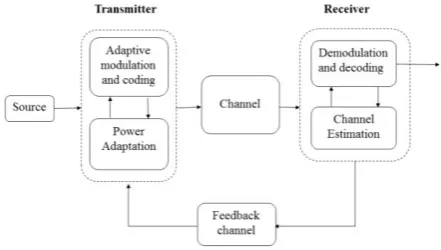
lifetimes emphasizes the importance of improving their energy efficiency [4]. Consequently, energy-aware algorithms that maximize the network lifetime are sought-after. In order to efficiently use energy, transmission schemes should be able to adapt to channel conditions through estimation and global feedback.
Adaptive modulation (AM), or link adaptation, allows for dynamic adjustment of transmission parameters to radio link conditions, such as available power level, channel path loss, signal interference and sensitivity of the receiver [5]. The parameters for adjustment can include: symbol rate, modulation schemes or constellation size, transmit power, and coding parameters [6]. These parameters can be varied either individually or jointly, according to channel conditions and quality of service (QoS) requirements. More recently [7] a “cognitive approach” is formalized for WSNs where global context information is used to optimize network performance at all layers. This new paradigm applies to this paper also for the special case where networking requirements are simplified and limited to lower layer performance to maximize node availability.
This paper first applies AM to single-hop WSNs. Then it proposes an Adaptive Sleep with Adaptive modulation (ASAM) algorithm for minimizing energy expenditure and enhancing the network lifetime. The ASAM algorithm dynamically changes the modulation scheme while adjusting the node sleep periods and power levels. We investigate several variations of these schemes and analyze and compare their performance under various channel conditions based on extensive computer simulations. Moreover, the power allocation problem is extended to multi-hop networks, where the algorithms are tested and evaluated under various fading scenarios.
The paper is organized as fellows: Sections II and III present the system model and the energy optimization problem, respectively. In Sections IV and V, AM, AMI and ASAM protocols are applied multi-hop relay networks. Finally, the simulation results are presented and analyzed in Section VI, followed by conclusions in Section VII.
2.
SYSTEM MODEL
2.1
System Architecture
process, delay and error can occur, impairing the accuracy of the estimates. However, in this paper, the impact of CSI data delay and estimation error is not taken into consideration.
Figure 1: Adaptive Feedback System Model
2.2
BER Approximations
In this paper, some results presented in [8, 9] will be used for the AM scheme. Readers can refer to this reference for detailed derivations. The spectral efficiency is defined as the average data rate per unit bandwidth (
R B
/
). The transmission rates are determined as
log [
2( )]
r
M
(bits/symbol), where
is the signal to noise ratio (SNR).The spectral efficiency for the discrete rate case is given by [8]:
1
1
0
( )
i
i
N i i
R
r
p
d
B
(1)where are the adaptive discrete rates determined by the modulation schemes.
The transmit power is restricted by an average transmit power constraintP:
(2) where p() is the probability density function of the SNR. With Gray bit mapping, the BER expression of square M-QAM schemes can be approximated as a function of the SNR and the constellation size M [10, 11, 12]:
2
2 1
1 1.5
log 1
MQAM
P
BER erfc
M M
P M
(3)
As this expression cannot be easily solved, the following approximation is considered [13]:
1.5 0.2
1
MQAM
P
BER exp P
M
2.3
Variable-Rate Variable-Power
Adaptation Policy
To formulate the variable-rate modulation problem, we consider a family of MQAM modulation schemes. The spectral efficiency is parameterized by the average transmit power and the BER, which lead to the expression for the constellation size as a function of the received SNR [14]:
1.5
( )
1
(5
)
P
M
ln BER
P
(5)The transmit power can be adapted to compensate for the channel fading. The goal is to maintain a fixed BER and equivalently, a constant received SNR. By introducing a power control technique to determine the power level needed for a successful transmission, power control values are formulated by rearranging equation (5) in terms of P( )
P
. We
then obtain the expression of the normalized power control factor as:
ln 5 ( 1)
( )
1.5
BER M
P P
(6)
3.
ENERGY OPTIMIZATION
A network with a fixed energy budget is defined as an energy-constrained network. WSN is one example of energy constrained networks. Sensor nodes in the network are usually battery-driven devices. Therefore, nodes must be able to operate for a long period of time without replacing the battery. Consequently, energy optimization for the communication processes becomes more crucial. It is necessary to understand the tradeoff between the system performance and the amount of energy that can be used for each process.
Recent research proposes the concept of energy-aware protocols to control the power levels during transmission [14]. One of the essential ideas in these protocols is to power down the nodes when they are not performing any tasks. This is due to the fact that in WSNs, nodes normally need to be communicating only for a short period of time; thus a high degree of redundancy usually exists in network topology [15]. It is possible to design wireless communication protocols to minimize energy consumption by letting the nodes sleep for a maximum period of time. Adaptive sleep (AS) technique, therefore, has been proposed so that node sleep times can be adjusted based on current fading conditions [16]. Most of the time when there is no communication, nodes are powered down and operated at the minimum power level. This stand-by power can be orders of magnitude lower than the active power. In energy-constrained networks, the total amount of energy available for a node is limited. In order to avoid frequent battery replacement for the sensor nodes, reducing energy expenditure during transmission is crucial. The general formula of energy consumption for a given node can be expressed as:
E
P T
(7),where P is the power level and T is the transmission time. In this paper, we consider four operation modes with different power levels for the sensor nodes:
-Idle mode: Here, the CPU maintains low activities. The radio transmission is off. Therefore, the current consumption in this mode is lower than in both the transmission and the active modes, but higher than the sleep mode.
• Sleep mode: After the data is successfully delivered, the node hibernates. Most node components are powered down and placed on stand-by to save energy. To wake up the transmitter and CPU again, it only needs a clock-type signal. The power consumption in this mode is the lowest among the four modes.
4.
ENERGY-AWARE MAC LAYER
PROTOCOLS
4.1
Basic Reference MAC Layer Protocol
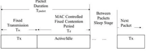
We define here a reference model for the medium access control (MAC), in which the active/idle duration are pre-allocated by the MAC layer’s contention period to ensure that the previous transmission is completed before the next one can take place. During this contention period, the node can operate either in the active mode with high CPU activities or in the idle mode with low CPU activities. Obviously, the active stage requires higher power level than the idle stage, but since the radio transmission is off, the power levels are much smaller compared to the transmission stage. The contention period gives extra room for the channel to deliver the previous packet and prepare itself for the next one. After the fixed contention period, node enters the sleep stage and wait for the next transmission.
The sleep stage, on the other hand, is the time interval between transmissions. It is also known as the “hibernation stage” to reduce energy consumption.
[image:3.595.55.294.524.610.2]The MAC layer protocol fixes the time of channel occupation for one transmission. It also pre-allocates the durations of the node transmission, active and idle stages, giving no freedom for energy adaptation. As illustrated in Figure 2: Time allocation in a reference MAC layer protocol, every time the node detects a packet waiting to be transmitted, the protocol wakes up the node and sets the fixed durations for the transmission, active and sleep stages.
Figure 2: Time allocation in a reference MAC layer protocol
The total consumed energy (
c
E ) consists of: Transmission energy (
tx
E ), Active energy (
E
active), Idle energy (E
idle), and Sleep energy (E
sleep).The total transmission time required for one packet (
T
packet)
and the contention period (
T
d) are pre-determined by the reference MAC layer protocol.4.2
Adaptive Modulation Mode (AM)
Adaptive modulation dynamically changes the data rate according to the channel condition. This normally varies the transmission duration to be less than the pre-allocated MAC transmission period. As illustrated in
Error! Reference
source not found.
(a), the node first switches to the active stage after transmission. It then enters the idle stage which has further reduced the power level compared to the other two stages. Note that the time for the transmission stage is controlled by AM while the node idle duration is still controlled by the MAC layer protocol. The overall energy consumption is calculated by considering the three types of energy expenditure in the network:
(8)
where is the transmit power; is the adaptive transmission time with is the packet length and being the AM rate; is the transmission energy. is the active power; is the time for the node operates in active stage, which varies in line with ;
is the active energy. is the idle power; is the fixed idle time determined by MAC layer protocol; is the idle energy. Also note that , and .
4.3
Adaptive Modulation with Adaptive
Idle Period (AMI)
In AM, the node operates in the active mode after the transmission when the CPU still has high activities, which might include executing back-stage programs and/or storing information in the memory. However, in WSNs, there is no need for the node to maintain a high volume of activities after each transmission. Instead, it can operate in idle mode immediately after the transmission with minimum CPU activities (see
Error! Reference source not found.
(b)). This offers additional improvement in energy efficiency. This process is called Adaptive Modulation with Idle Mode (AMI). Its total energy consumption is determined as:Similarly, is the transmit power; is the adaptive transmission time, is the packet length and is the AM rate; is the transmission energy. is the idle power; is the adaptive idle time; is the fixed node idle time; is the idle energy. In this case,
4.4
Adaptive Sleep with Adaptive
Modulation (ASAM)
For further optimization in energy consumption, the network can consider employing MAC layer adaptive sleep which has been studied to improve energy efficiency in WSNs [17]. The protocol sets the duty cycle for the contention period and
𝑰=
+
= × + × + ×
= × + × ( ) + ×
adaptively adjusts the sleep time. Therefore, instead of remaining in the active and idle stage, it can stay in the sleep stage after the contention period until the next packet is ready to be transmitted.
As shown in
Error! Reference source not found.
(c), the MAC layer still allocates the same amount of idle period to ensure the previous packet is successfully delivered. However, instead of staying in the active or idle stage for a while, the node is put into the sleep stage right after the pre-allocated contention period
T
d . In other words, the additional active or idle stage is not necessary for this algorithm. The total time for completing one packet is adaptively adjusted.Therefore, not only the transmission time is adapted by AM, but also the sleep time is varied by AS. The energy consumption formula in this case becomes:
(10)
Note that in this case, is the sleep power; is the adaptive sleep duration; is the sleep energy dynamically controlled by AS protocol.
(a) AM
(b) AMI
(c) ASAM
Figure 3: Illustration of AM, AMI and ASAM protocols
𝑺 =
+ + 𝒔
= × + × + 𝒔 × 𝒔
5.
ENERGY OPTIMIZATION FOR
MULTI-HOP NETWORKS:
APPLICATION TO A TWO-HOP
NETWORK
In the previous section, the node energy consumption per packet transmission was discussed for single-hop WSNs. However, a typical connection between the source node and destination node in a WSN system usually uses several relay nodes through multi-hop protocols since network lifetime is impacted not only by the node energy consumption statistics but also by loss of connectivity [17, 18]. Here we will extend the analysis to two-hop networks, where the focus is on the lifetime of the overall network instead of the lifetime of a single node. Error! Reference source not found. shows an illustration of a multi-hop connection in a WSN with varying channel conditions.
[image:5.595.58.276.322.449.2]In particular, this work is interested in two types of multi-hop networks: 1) relay networks where source data is transmitted to the destination via relay nodes, and 2) multiple-link networks where multiple wireless communication links are formed by several independent sources and destinations.
Figure 4: Example of a multi-hop relay network
[image:5.595.309.548.434.693.2]In the same WSN, communication links are usually subject to different channel conditions [19]. Let’s consider a n-link relay network model, where the source, relay and destination nodes form two wireless channels. Figure shows an example of a path composed of a source, relay and destination nodes.
Figure 5: Example of a two-hop link Model
The network performance is constrained by the total available energy. Although the amount of energy is fixed, the necessary transmit power allotted to each node is adaptively adjusted to achieve minimum network energy consumption. We introduce a power allocation factor
i for a given node i. It is defined as the percentage of the total average power allocated to the node; hence
i must satisfy . The total energy is divided between the source node and the relay nodes.i
should satisfy the following energy constraints:, (11)
(12)
We denote the energy consumption in link i as Ei and the link
lifetimes as Ti. In addition, it is assumed that when the energy
allocated to a given node has been exhausted, the network is
considered as “dead” and reaches its lifetime limit. The network lifetime is defined as the period of time in which all nodes are able to transmit data. The optimal network lifetime T* is expressed as:
(13)
where
* is the optimal power allocation vector that contains the power allocation factors for all links when the network lifetime is maximized. Considering the energy consumption, we can formulate the problem by calculating the minimum energy consumption in the entire network subject to optimal power allocation:* *
1
,
2,...,
,..
min(
(
i.
.
totalhops)
)
E
max E E
E
E
(14)
Thus, by solving the optimal network energy consumption problem, the optimal power allocation factors are determined. As the analytical solution is difficult to obtain, the optimal allocation factors will be determined by exhaustive search through simulation.
6.
COMPUTER SIMULATION RESULTS
AND DISCUSSIONS
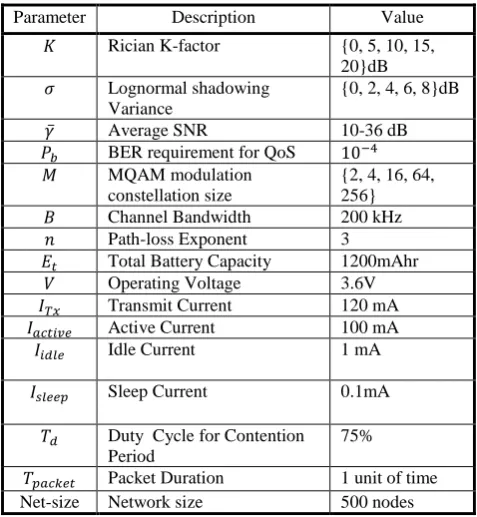
[image:5.595.56.293.533.564.2]In the computer simulations below, we consider 6 modulation schemes: no transmission, BPSK, QPSK, 16QAM, 64QAM and 256QAM. For illustration purposes, the target BER was set to , and the average SNR was varied from 10dB to 36dB. The fading channel is characterized by a Rician (with a Rician factor K) or a Log-Normal shadowing distribution (with standard deviation σ), respectively. The following table summarizes the simulation parameters.
Table 1. Simulation Parameters
Parameter Description Value
Rician K-factor {0, 5, 10, 15, 20}dB Lognormal shadowing
Variance
{0, 2, 4, 6, 8}dB
Average SNR 10-36 dB
BER requirement for QoS MQAM modulation
constellation size
{2, 4, 16, 64, 256} Channel Bandwidth 200 kHz Path-loss Exponent 3
Total Battery Capacity 1200mAhr Operating Voltage 3.6V
Transmit Current 120 mA
Active Current 100 mA
Idle Current 1 mA
Sleep Current 0.1mA
Duty Cycle for Contention Period
75%
Packet Duration 1 unit of time Net-size Network size 500 nodes
6.1
. Performance of AM, AMI and ASAM
without power control
6.1.1
Influence of the number of available
modulation schemes:
AMI, and ASAM with no power control. Recalling the energy consumption formulas discussed in Section Error! Reference source not found., the node lifetime of AM, AMI, and ASAM is calculated based on the different operating stages required by each algorithm. At each simulation run, 500 nodes are deployed randomly and we analyze the nodes lifetime for successfully delivering a target number of packets using the adaptive discrete rate continuous power policy.
[image:6.595.327.555.188.513.2]The node lifetime achieved by the three algorithms under different fading conditions are shown in Figures. 6 and 7 for Lognormal shadowing and Rician fading, respectively. Here we have studied the influence of the number of modulation stages available. For example, 3 modulation stages mean that, at a given time, the AM algorithm will choose one modulation scheme among: No transmission, BPSK or QPSK. 6 modulation stages mean that all modulation schemes are available (i.e., no transmission, BPSK, QPSK, 16QAM, 64QAM and 256QAM).
Figure 6: Impact of modulation stages on node lifetime under Lognormal shadowing when σ = 4dB
Figure 6 indicates that the higher the number of stages available, the longer the node lifetime. This is due to the fact that the availability of high-level modulation schemes enables the system to choose the ones that allow the highest spectral efficiency and therefore the lowest transmission time. For low SNRs, the performance does not depend on the number of stages because, in this case, the lowest modulation schemes (e.g., no transmission or BPSK) are likely to be used (because of the poor channel conditions in this case).
6.1.2
Comparison between the proposed
protocols under different channel conditions:
It can be seen from Figs. 6 that the proposed ASAM algorithm consistently outperforms the AM technique. Nodes can operate up to 221 days using ASAM while the longest node lifetime using AM is 42 days only. In addition, AMI slightly improves the node lifetime compared to AM. At the high SNR region, AMI outperforms AM by approximately 10 days. In AM, the node is first active after the transmission stage, then switches to the idle stage, and finally enters the sleep stage. In AMI, the active stage is replaced by the idle stage since the processor only requires minimum functionality. Therefore, this portion of the energy is reduced from active energy to idle energy. However, since the power level at the sleep stage is the least, it would be desirable to have the node
stay in this stage for a maximum period of time. The ASAM algorithm provides good adjustment of nodes sleep duration, and therefore further enhances the energy efficiency. The main difference between ASAM and AM is that the former enters the sleep stage right after the contention period (that is pre-allocated by the MAC layer protocol), while the latter still stays active for a certain period of time before entering the contention period. The significant difference between the sleep power and active power can considerably affect node lifetime, as illustrated in the figures.
(a) Lognormal Shadowing: σ = 2, 4, 8dB
[image:6.595.55.277.282.465.2](b) Rician Fading: K = 0, 10, 20dB
Figure 7. Node lifetime simulation: comparison of 6 stages ASAM, AMI, and AM for (a) Lognormal
shadowing and (b) Rician Fading.
Figures 7.a and 7.b display the node lifetime as a function of σ and K, for Lognormal shadowing and Rician fading effects, respectively. Fig. 7.a shows that for each algorithm, under a given average SNR, stronger Lognormal shadowing (i.e., higher σ) yields a shorter node lifetime. In other words, the energy cost is reduced when the network operates in a good channel condition. The behavior is similar for the Rician fading case (Fig. 7.b). The node can operate longer when the fading in the wireless channel is minor (i.e., higher K). Moreover, the figures demonstrate that the node lifetime is heavily dependent on the average SNRs in the network. For the same channel fading condition, increasing the average
10 12 14 16 18 20 22 24 26 28 30 32 34 36
0 50 100 150 200 250
Lognormal shadowing when = 4 dB
Average SNR (dB)
N
o
d
e
L
if
e
ti
m
e
(
d
a
ys)
3 Stages ASAM 4 Stages ASAM 5 Stages ASAM 6 Stages ASAM 3 Stages AMI 4 Stages AMI 5 Stages AMI 6 Stages AMI 3 Stages AM 4 Stages AM 5 Stages AM 6 Stages AM
10 12 14 16 18 20 22 24 26 28 30 32 34 36
0 50 100 150 200 250
Lognormal shadowing when = 0 dB
Average SNR (dB)
N
o
d
e
l
if
e
ti
m
e
(
d
a
ys)
6 Stages ASAM ( = 2dB) 6 Stages ASAM ( = 4dB) 6 Stages ASAM ( = 8dB) 6 Stages AMI ( = 2dB) 6 Stages AMI ( = 4dB) 6 Stages AMI ( = 8dB) 6 Stages AM ( = 2dB) 6 Stages AM ( = 4dB) 6 Stages AM ( = 8dB) Adaptive Modulation
with Idle Mode
Adaptive Modulation Adaptive Modualtion with Adaptive Sleep
10 12 14 16 18 20 22 24 26 28 30 32 34 36
0 50 100 150 200 250
Rician Fading when K = 20 dB
Average SNR (dB)
N
o
d
e
l
if
e
ti
m
e
(
d
a
ys)
6 Stages ASAM (K = 20dB) 6 Stages ASAM (K = 10dB) 6 Stages ASAM (K = 0dB) 6 Stages AMI (K = 20dB) 6 Stages AMI (K = 10dB) 6 Stages AMI (K = 0dB) 6 Stages AM (K = 20dB) 6 Stages AM (K = 10dB) 6 Stages AM (K = 0dB) Adaptive Modulation
with Idle Mode
[image:6.595.330.556.388.591.2]SNR extends the node lifetime. This trend applies to both Lognormal shadowing and Rician fading channel conditions. For strong fading cases, a poor SNR can substantially degrade node lifetime.
Although the figures indicate that for all the algorithms, the sensor nodes can operate longer with smaller channel fading and larger SNRs, the channel fading conditions and average SNRs show very distinct impacts on energy consumption for different algorithms.
For AM, the channel condition has a bigger impact on the node lifetime at low SNRs than at high SNRs. As the average SNR increases, the lifetime gap between different fading conditions becomes smaller.
On the other hand, AMI puts the node into the idle stage immediately after transmission. Even under poor channel conditions where a lot of retransmissions occur, the node only spends the idle power after the retransmission, which is normally much smaller than active power.
The channel fading conditions and average SNRs have significant impacts on the node lifetime in ASAM. Compared to AM, the performance of the ASAM algorithm is more notably influenced by the average SNR. The difference in node lifetime is approximately 120 days between the lowest and the highest SNRs for ASAM, while for AM, the difference is less than 30 days.
Under low average SNR, a bigger σ indicates both a higher chance of retransmission and a higher chance of transmission with a larger data rate. For AMI and ASAM, the retransmission cost is essentially reduced; hence the energy saving gained from higher-rate transmission outweighs the downside, i.e., the larger σ, the longer node lifetime, as shown in the plots. For AM cases, on the other hand, a smaller σ consistently yields better performance relative to a larger σ. Such phenomenon happens because the retransmission cost for AM is considerably higher than for AMI and ASAM, due to the active power level used when retransmission occurs. The disadvantage of having larger σ outweighs the advantage in such cases.
Moreover, under a high average SNR, the node is already transmitting data with a high rate. Increasing σ, therefore, might contribute to a small degree to a better transmission speed, but would increase the likelihood of having low instantaneous SNR, i.e., a low transmission rate and more energy consumption. As reflected in the figures, smaller σ always gives longer node lifetime in the high average SNR regions.
6.2
Performance of AM, AMI and ASAM
with power control
Here a power control factor is introduced to adjust the value of transmit power within the same level of modulation. Based on Equation (7), the optimal values of the power adaptation factor are derived allowing the power and rate to be jointly adapted according to channel conditions.
The node lifetime is measured for the following six cases: 1) Adaptive Sleep combined with Adaptive modulation under Power Control (ASAM-PC), 2) Adaptive Sleep combined with Adaptive modulation NO Power Control (ASAM), 3) Adaptive Modulation with Idle mode under Power Control (AMI-PC), 4) Adaptive Modulation with Idle mode with NO Power Control (AMI), 5) Adaptive Modulation under Power Control (AM-PC), and 6) Adaptive Modulation NO Power Control (AM).
Figure 8 indicates that the power control adaptation policies perform better in the case of ASAM. This superior performance is due to the fact that ASAM has very good adaptation capability given the algorithm’s ability to dynamically adjust the operating durations for both the transmission stage and the sleep stage.
6.3
Multi-hop power optimization
The proposed multi-hop adaptive power allocation policy (Section 5) is employed for a multi-hop network. The network lifetime depends on the energy consumption of all wireless links along the communication path. Although the total available energy in the network is finite, the power allocated to each node can be adjusted to achieve optimal transmission quality with minimal energy consumption.
(a) Lognormal Shadowing: σ = 2dB
[image:7.595.328.549.238.546.2](b) Rician Fading: K = 10dB
Figure 8: Power control impacts on node lifetime using 6 stages ASAM, AMI and AM under (a) Lognormal shadowing: σ = 2dB and (b) Rician Fading: K = 10dB.
For illustration, we simulated a 500-node sensor network based on two-hop relaying. At each simulation run, a new network is randomly generated. The power allocation policy is responsible for allotting the optimal power according to the instantaneous fading information of each link.
In general, the allocated power is biased to the link with poorer channel condition. This is to ensure operations of all links in the network are maintained simultaneously for the maximal period of time. Our scheme grants more energy to the link located in poorer channel conditions so that by extending its lifetime, the lifetime of the entire network is extended. Figure 9 displays the node lifetime for σ1 = 2dB, σ2 = 8dB, respectively. The optimal power allocation scheme is compared to the case where the total energy is evenly divided between the nodes (i.e., the source and relay nodes are allocated equal portions of the total available energy,
10 12 14 16 18 20 22 24 26 28 30 32 34 36 0
50 100 150 200 250
Average SNR (dB)
N
od
e
lif
et
im
e
(d
ays)
Node lifetime in lognormal shadowing when = 2 dB
ASAM-PC ASAM AMI-PC AMI AM-PC AM
10 12 14 16 18 20 22 24 26 28 30 32 34 36
0 50 100 150 200 250
Average SNR (dB)
N
od
e
lif
et
im
e
(d
ays)
Node lifetime in Rician Fading when K = 10 dB
regardless of their channel conditions). It can be seen from the Figures that improved network lifetime is obtained for all algorithms that use optimal power allocation. The improvement is more notable for ASAM. As the node lifetime for ASAM is more subject to channel conditions than AM, wisely allocating the energy to each link according to its fading condition is essential for enhancing the energy efficiency of the entire network in ASAM. Moreover, the results indicate that a more considerable increment can be achieved under more distinct fading conditions between the two links. Also, power allocation with the AM scheme is shown to perform better at low SNR regions than at high SNR region; with ASAM, the power allocation algorithm is found to improve the network lifetime more at high SNRs. For AM, variations in channel fading conditions have a minor influence on energy consumption. In low SNR cases, however, node lifetime is more sensitive to fading conditions so energy resources need to be more carefully allocated to improve energy efficiency. Conversely, for ASAM, the channel fading has more significant impacts on the node lifetime under high average SNRs. Therefore, adaptive power allocation has a higher impact as SNR increases in this scenario.
Figure 9: Impact of power allocation on a two-hop network under Lognormal shadowing: σ1 = 2dB, σ2 =
8dB.
7.
CONCLUSIONS
This paper investigated a number of link adaptation algorithms for energy constrained wireless sensor networks and introduced lower cognition levels that allowed nodes to use information about neighboring nodes and channel conditions to optimize energy use and maximum network life time in general. The algorithms have been evaluated in terms of network lifetime and the energy consumption. The ASAM algorithm has been shown to outperform AMI and AM algorithms in terms of network lifetime and energy efficiency. In the case of multi-hop networks, it was shown that an optimized power distribution between hops outperforms evenly distributed power. Future work will consist of providing an in-depth analytical analysis for the proposed schemes for the various scenarios discussed in this paper
.
8.
REFERENCES
[1] S. G. Cui, et al., "Energy-constrained modulation optimization," IEEE Transactions on Wireless Communications, vol. 4, pp. 2349-2360, Sep 2005. [2] S. Phoha, et al., Sensor network operations. Hoboken,
N.J. and Piscataway, N.J. Wiley; IEEE Press, 2006. [3] T. Yan, et al., "Design and optimization of distributed
sensing coverage in wireless sensor networks," ACM Trans. on Embedded Computing Systems, vol. 7, 2008.
[4] I. F. Akyildiz, et al., "Wireless multimedia sensor networks: A survey," IEEE Wireless Communications, vol. 14, pp. 32-39, Dec 2007.
[5] A. Goldsmith, Wireless communications. Cambridge, New York: Cambridge University Press, 2005.
[6] M.S. Alouini and A.J. Goldsmith, "Adaptive modulation over Nakagami fading channels," Wireless Personal Communications, vol. 13, pp. 119-143, May 2000. [7] E. Bdira & M. Ibnkahla, “Performance Modeling of
Cognitive Wireless Sensor Networks Applied to Environmental Protection,” IEEE GLOBECOM, (2009 pp. 1-6).
[8] A. J. Goldsmith and P. P. Varaiya, "Capacity of fading channels with channel side information," IEEE Transactions on Information Theory, vol. 43, pp. 1986-1992, Nov 1997.
[9] T. Ue, et al., "Symbol rate and modulation level-controlled adaptive modulation TDMA TDD system for high-bit-rate wireless data transmission," IEEE Trans. Veh. Technology, vol. 47, pp. 1134-1147, Nov 1998. [10]Q. W. Liu, et al., "Cross-layer combining of adaptive
modulation and coding with truncated ARQ over wireless links," IEEE Transactions on Wireless Communications, vol. 3, pp. 1746-1755, Sep 2004. [11]B. Classon, et al., "Channel coding for 4G systems with
adaptive modulation and coding," IEEE Wireless Communications, vol. 9, pp. 8-13, Apr 2002.
[12]S. Nanda, et al., "Adaptation techniques in wireless packet data services," IEEE Communications Magazine, vol. 38, pp. 54-64, Jan 2000.
[13]A. Y. Alemdar, "Link Adaptation For Energy Constrained Networks," Master of Science (Engineering), Department of Electrical and Computer Engineering, Queen's University, Kingston, 2008. [14] B.M. Sadler, "Fundamentals of energy-constrained
sensor network systems," IEEE Aerospace and Electronic Systems Magazine, vol. 20, pp. 17-35, 2005. [15]Y. T. Hou, et al., "On energy provisioning and relay node
placement for wireless sensor networks," IEEE Transactions on Wireless Communications, vol. 4, pp. 2579-2590, Sep 2005.
[16] J. Van Greunen, et al., "Adaptive Sleep Discipline for Energy Conservation and Robustness in Dense Sensor Networks," presented at the 2004 IEEE International Conference on Communications, 2004.
[17]P. Agrawal and N. Patwari, "Correlated Link Shadow Fading in Multi-Hop Wireless Networks," IEEE Transactions on Wireless Communications, vol. 8, pp. 4024-4036, Aug 2009.
[18]M. Ilyas and I. Mahgoub, Handbook of sensor networks : compact wireless and wired sensing systems. Boca Raton: CRC Press, 2005.
[19] D. P. J. Van Greunen, A. Bonivento, J. Rabaey, K. Ramchandran, A.S. Vincentelli, A.S.; , "Adaptive Sleep Discipline for Energy Conservation and Robustness in Dense Sensor Networks," presented at the IEEE International Conference on Communications, 2004
10 12 14 16 18 20 22 24 26 28 30 32 34 36
0 50 100 150 200 250
Two Links channel conditions: 1 = 2 dB, and 2 = 8 dB
Average SNR (dB)
N
et
w
or
k
lif
et
im
e
(ye
ar
s)