Path Planning of an Autonomous Mobile Robot using
Directed Artificial Bee Colony Algorithm
Nizar Hadi Abbas,
PhD Electrical EngineeringDepartment College of Engineering University of Baghdad, Iraq
Farah Mahdi Ali
Electrical Engineering Department College of Engineering University of Baghdad, Iraq
ABSTRACT
This paper describes the problem of offline autonomous mobile robot path planning, which is consist of generating optimal paths or trajectories for an autonomous mobile robot from a starting point to a destination across a flat map of a terrain, represented by a 2-D workspace. An improved algorithm for solving the problem of path planning using Artificial Bee Colony algorithm is presented. This nature-inspired metaheuristic algorithm, which imitates the foraging behavior of bees around their hive, is used to find the optimal path from a starting point to a target point. The proposed algorithm is demonstrated by simulations in three different environments. A comparative study is evaluated between the developed algorithm, the original ABC and other two state-of-the-art algorithms. This study shows that the proposed method is effective and gets trajectories with satisfactory results.
General Terms
Nature-inspired algorithm, Heuristic algorithms
Keywords
Autonomous robots, Holonomic robot, Path planning, Optimization methods, Artificial bee colony algorithm
1.
INTRODUCTION
The field robot path planning was launched at the middle of the 1960’s. Robot path planning is an important problem in navigation of mobile robots. The aim is to find an optimal and collision-free path from a predefined start position to a target point in a given environment. Generally, there are many paths for robot to reach the target, but in fact, the best path is selected according to some guideline. These guidelines are: shortest distance, least energy consuming or shortest time with the shortest distance is the most adopted criteria. Path planning can be seen as an optimization problem since its purpose is to search for a path with shortest distance under certain constraints such as the given environment with collision-free motion [1]. In the past several decades, research on optimization algorithms has covered a wide area of researchers' attention. Optimization methods and algorithms can be classified in many types, but the simplest way is to look at the nature of the algorithm, and this grouped them into deterministic and stochastic [2, 3] where deterministic techniques depend on the mathematical nature of the problem, while stochastic techniques do not depend on the mathematical properties of a given function and are hence more appropriate for finding the global optimal solutions for any type of objective function. However, the weaknesses of first technique are its dependence on gradient, local optima and inefficient in large-scale search space and cannot solve discrete functions. Stochastic techniques are considered to be more users friendly. As many real-world optimization problems become increasingly complex, using stochastic
methods is inevitable. These algorithms have been found to perform better than the classical or gradient-based methods, especially for optimizing the non-differentiable, multimodal, and discrete complex functions. Some effective stochastic techniques that mimic the behaviors of certain animals or insects (birds, ants, bees, flies and even germs!) and called Nature-Inspired Algorithms have been developed since 1980s. Currently, these nature-inspired paradigms have already come to be widely used in many areas in engineering fields[4,5].Some of these algorithms are Particle Swarm Optimization(PSO)[6], Ant Colony Optimization (ACO) [7] and Artificial Bee Colony (ABC)[8].
The Artificial Bee Colony (ABC) optimization is one of the most-recent population based (swarm intelligence based) meta-heuristic algorithms, which simulate the foraging behavior of honey bee colonies. It proposed by D. Karaboga [8] in 2005 for real-parameter optimization problems. Numerical comparisons demonstrated that the performance of the ABC algorithm is an efficient algorithm when compared with other population-based algorithms through an advantage of employing fewer control parameters. Due to its simplicity, flexibly and ease of implementation, the ABC algorithm has captured much attention and has been applied to solve many practical optimization problems [9].
In this paper, an improved version of the ABC algorithm called Directed Artificial Bee Colony (DABC) is proposed. DABC is used to solve the path planning problems by making use of current direction of the best bee and guide the other bees toward this direction.
The rest of this paper is organized as follows: section 2 describes path planning and problem formulation; Section 3 describes the standard ABC algorithm; Section 4 describes the proposed DABC algorithm; Section 5 explains robot path planning using DABC, and the simulation results are shown in section 6. Finally, section 7presents the conclusion of the paper.
2.
PATH PLANNING AND PROBLEM
FORMULATION
Robot Path planning (RPP) is one of the important aspects in robot navigation research. Depending on the environment where the robot located in; RPP can be classified into two types:
1) RPP in static environment which has fixed obstacles. 2) RPP in dynamic environment which has both fixed and moving obstacles.
Each of these two types could be further subdivided into a sub-group:
2) Local Path Planning (LPP): is usually constructed online when the robot avoids the obstacles in a real time environment [10].
In this paper, global path planning is adopted where the environment is static and totally known. Constructing a model for the environment is important issue; an appropriate representation of the terrain is needed to generate a sufficiently complete map of the given surroundings that the robot will encounter along its route. The mobile robot is defined as a point object in the 2-D space. Since the robot reduced to a point, each obstacle must be inflated by the size of the robot’s radius to compensate. Each obstacle can be represented by polygon surrounded by a circle. Obstacles are finite in size and do not overlap and have a safety zone which is the region around the obstacle that the mobile robot must avoid. As the obstacle is of an irregular shape, the radius must be one-half of the longest side of the obstacle plus the robot's radius.
3.
STANDARD ABC ALGORITHM
Artificial Bee Colony (ABC) algorithm invented by D. Karaboga [8] is a relatively new population-based algorithm; it is a nature-inspired metaheuristic algorithm, which imitates the foraging behavior of bees. ABC as a stochastic technique is easy to implement, and could easily be modified and hybridized with other metaheuristic algorithms [11]. In real colonies, including bees, some tasks are performed by specialized individuals. These specialized bees try to maximize the nectar amount stored in the hive using efficient organization.
The minimal model of swarm-intelligent forage selection in a honey bee colony which the ABC algorithm simulates consists of three kinds of bees: employed bees, onlooker bees and scout bees. Half of the colony consists of employed bees, and the other half includes onlooker bees. More bees should send to high-quality sources, and fewer bees should be sent to low-quality sources or even abandoned. At the beginning, the colony sends employed bees to rich flower patches. These bees get flower's nectar and carry them to the hive. When they come back to the hive, unload their nectar and go to a certain area in the hive called ‘dance floor’ to share their information with other bees. The communication is performed by a special dance. If the region visited by an employee is nearby, it performs "round dances" in the hive, and if not, the bee performs a "waggle dance". Round dance contains information about the nectar quality of a visited flower patches so the other bees can find its location by their smelling sense when they get out of the hive.
Waggle dance contains three pieces of information about the flower patch: its direction with respect to Sun, its distance from the colony, and the nectar amount [12]. Onlooker bees watch the dances in the hive and choose the best flower patches to go for. Indeed, flower patches which have higher qualities attract more bees than lower quality flower patches. Employed bees that their visited region is abandoned because of low quality have two options: go to the dance floor and watch dances of other bees then go to a flower patch as an onlooker bee, or it search around the hive spontaneously as a scout bee for a new food source due to some internal motivation or possible external clue [13].
ABC algorithm can be summarized as in the following subsections [13]:
3.1 Population initialization
A population of FN individuals is produced randomly, which is equal to the number of food sources. Each solution (i = 1, 2… FN) representing an individual is a D-dimensional vector. Here, D is the number of optimization parameters. Each solution can be generated by Eq. (1)[14]:
(1)
where i = 1, 2… FN, j = 1, 2… D. and are the lower bound and upper bound ofthe parameter j, respectively. Next, the fitness of each food source is evaluated by
=
(2)
where is the fitness value of the solution i.
3.2 Employed bee phase
At this stage, a new candidate solution is produced for the employed bee of food source (only one parameter of the solution is updated by using Eq. (3) :
(3)
where k ∈[1...FN] and j ∈[1...D] are random numbers, and k has to be different from i, and is a random real number in the interval of [−1, 1]. After producing a new food source (solution) , it will be evaluated and compared with immediately. Then a greedy selection process is applied by comparing the fitness of both solutions produced via Eq. (2). If the fitness of solution is better than or equal to that of the solution , will be replaced with and the individual will become a new member of the population and the abandonment counter of the employed bee is reset. Otherwise, food source is kept unchanged and abandonment counter is increased by 1.
3.3 Onlooker bee phase
After all employed bees complete the search process; each onlooker bee chooses an employed bee to improve its solution with a probability value , which is calculated by roulette wheel using Eq. (4).
(4)
where is the fitness value of solution , which is proportional to the nectar amount of that food source.Obviously, the higher the , the more the probability of selecting the ith food source is. In the onlooker bees' phase, an artificial onlooker bee chooses its food source depending on the above mentioned probability value . After a food source for an onlooker bee is probabilistically chosen, a new neighborhood source is determined according to the Eq. (3) and its fitness value is computed. As in the employed bees phase, a greedy selection is applied.
3.4 Scout bee phase
Then a new solution is calculated for the scout bee by using Eq. (2) and the abandonment counter is reset. The scout bee, which a solution was produced for itself, becomes the employed bee. Therefore, scout bees in ABC prevent stagnation of employed bee population.
4.
DIRECTED ABC (DABC)
ALGORITHM
In standard ABC, finding a neighboring food source is defined by Eq.(3).As mentioned before in real bee colonies a waggle dance contains information that hive mates share; one of this information is the direction of the food source. So a method for guiding the bees either to left or right toward the current food source (for x-axis) and up or down to the current food source (for y-axis) and keep this direction as long as the fitness increased. While the coefficient in the Eq. (3) is a uniformly distributed random number in the range of [−1, 1], a new is defined as follows:
∈
∈ (5)
First let in the employed bee phase and check if the solution improved, then keep this phi for the onlooker bee in next phase to keep the same direction. Otherwise if the fitness does not improved in the employed phase, this lead to swap the current direction and choose . This will increase the chance for the onlooker bee to head to the right direction. Small modification introduced to the standard ABC Eq. (3) as shown below:
(6)
where abs stands for the absolute difference between the current food source and a neighbor one. Taking absolute value making sure that the signed phi (either or ) works properly.The procedure of directed artificial bee colony algorithm can be described in Algorithm 1.
Algorithm 1: Directed Artificial Bee Colony Algorithm
Step1: Initialize the population of solutions i = 1, 2….SN, j =1, 2…D). Evaluate the population, and iteration=1. Set coefficient (either or ).
Step2: Repeat
Step3: For each employed bee produce new solutions by using Eq. (3), then apply the greedy selection process and evaluate proper for the onlookers. If fitness for is better than then =0. Else = +1.
Step4: Calculate the probability values for the solutions by Eq. (4).
Step5: Produce the new solutions for the onlookers from the solutions selected depending on andevaluated , then apply the greedy selection process. If fitness for is better than then =0. Else = +1. Step6: Determine the abandoned solution, if =limit Then replace it with a new randomly produced solution by Eq. (1).
Step7: iteration=iteration+1, go to step 2 until iteration=MCN.
5.
ROBOT PATH PLANNING USING
DABC
The first step in using DABC algorithm is to make an initial path for robot from the starting point to the target. Since several obstacles situated in between, initial path has some breakpoints (two successive straight segments of the path meet each other), depends on the number of obstacles and the size of the environment. The created path is not optimal according to distance neither smoothness. The second step is using the proposed algorithm to find the optimal or near an optimal path. As stated before the environment would be 2D work space with circular obstacles. The mobile robot is represented as a dot by Cartesian coordinates (x,y) in the xy-plan. The problem's objective is to find the shortest path without violate any constrain, which is avoiding all obstacles present in the way. The optimization problem formulated to make up a discrete optimization problem, where the objective function aims to minimize the total path traveled by the mobile robot. It is given by:
(7)
where represent the Euclidian distance between the start and target points, is the number of breakpoints (trajectory change occurred).While the most important property of heuristic algorithms, including the ABC algorithm is that they are designed for the unconstrained optimization problems, they can also be adapted to the constrained optimization problems by using penalty. If a solution doesn’t satisfy the constraints, this solution is not acceptable, even if the value of the objective function is minimized [15]. The total function is called as fitness function. Namely, if constraints are in the feasible region, then the penalty function is equal to zero. Otherwise, the fitness function is penalized by a penalty function. Many researchers introduced different methods for representing a proper fitness function for finding an optimal path. In this work, a proposal of new expression for fitness function is introduced to enhance the smoothness of the robot's path. Mobile robot needs a portable power source; this maximizes the need for power saving by preventing the robot from making unnecessary turning and redundant movements. Consequently, minimizing the angles between the straight lines that connecting the breakpoints would be a second objective function (Eq. (8) and Eq. (9)) that the algorithm should be satisfied in addition to the first objective which is minimizing the distance (Eq.(7)).
(8)
The proposed fitness is formulated as follows,
(10)
To demonstrate the second objective function , a simple example for a path selection is taken. For Fig.1 let points (i+1) and (i+1) be next candidate break points to a point P(i) which belong to a path. Assuming that both points construct a feasible path, and there is a virtual line between breakpoint P(i) and the target. Both next points ( (i+1) and (i+1)) would have an angle with this line, namely the angles difference and respectivly. According to the previous assumption, the fittest one that satisfied the second objective function ( ) would be point (i+1) since it has smaller angle difference (angle error) and seems better headed toward the target. Generally, when comes to select a whole path consisting of many such points, a summation for all breakpoints angles would be done. The algorithm would choose the path with less angles error (path 1 in Fig.2).
6.
SIMULATION RESULTS AND
DISCUSSIONS
The environment used for the planning is a 10x10 unit less workspace. The unit meter (m) used in the simulations can be multiply by any scale (*10 for example). Starting point is (0,0) and target point is (10,10). MATLABR2011b programming language used to create the simulation code for path planning using 2.13GHz processor and 2 GB RAM. The following parameters is set: =2, =.5, =100 and =3 (case 1) and =4 (case 2 and case 3)
6.1
Case study 1: Environment with 4
obstacles
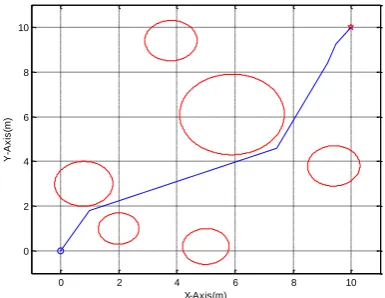
All obstacles' positions (center and radius) are listed in Table 1.The experiment has achieved a feasible solution; the best trajectory was achieved by DABC is illustrated in Fig.3. Via points: P1(2.3166,2.1589), P2(2.6423,2.5094), P3(6.0611,7.4974) and distance = 14.3589 using DABC. While best trajectory achieved by ABC in Fig 4. Via points: P1(3.5096,3.6183), P2(6.0706,7.6783), P3(7.2608, 8.6489) and distance=14.4311. Best distances achieved by GA and bacterial colony in [16] were 14.5087 and 14.3796 respectively.
6.2
Case study 2: Environment with 6
obstacles
All obstacles' positions (center and radius) are listed in Table 2. The best results for both algorithms: via points: P1(1.7716, 1.8519), P2(7.3059,4.7008), P3(9.8801,b), P4(9.9999,10.0) and distance=14.7986 by using DABC algorithm is shown in Fig.5. For ABC algorithm best results achieved were via points: P1(1.0,1.8083), P2(7.4317,4.6038) ,P3(9.1758,8.4092), P4(9.4817,9.2603) and distance=15.073 is illustrated in Fig.6. The best result achieved by chaotic bee swarm optimization algorithm in [17] was via points: P1 = (1.91891, 2.27910); P2 = (7.32502, 4.61828); P3 = (7.39433, 4.70942) with total distance equal to 14.8821.
6.3
Case study 3: Environment with 12
obstacles
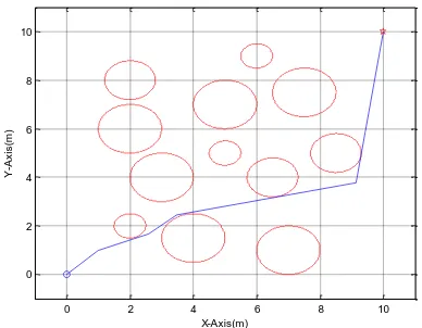
[image:4.595.61.272.274.657.2]All obstacles' positions (center and radius) are listed in Table 3. The best results for both algorithms: via points: P1(3.0106,2.0708), P2(8.2225,6.5937), P3(10.0,9.9393) ,P4(10.0,9.9391) and distance =14.4043 by DABC (Fig.7). Via points: P1(1.0,1.0), P2(2.5919 ,1.6850), P3(3.4649,2.4604), P4(9.1378 ,3.7687), distance =16.4274 by ABC (Fig.8). The best solutions achieved by bacteria colony and GA in [18] are 14.4035 and 14.4098 respectively.
Table 1: Definition of obstacles for the case study 1.
Obstacle No.
Radius Center(X,Y)
1 1 (4,1.5)
2 1 (2,3.5)
3 2 (7.5,6)
4 1.5 (3.5,7.5)
Figure 2: Two paths selection (summation angles
error).
[image:4.595.340.519.631.704.2]Table 2: Definition of obstacles for the case study 2
Obstacle No.
Radius Center (X,Y)
1 1 (.8,3)
2 .7 (2,1)
3 .8 (5,.2)
4 .9 (3.8,9.4)
5 1.8 (5.9,6.1)
6 .9 (3.8,9.4)
[image:5.595.329.522.82.231.2]Figure 6: Best results achieved by original ABC case 2
Table 3: Definition of obstacles for the case study 3
Obstacle No.
Radius Center
(X,Y)
1 .5 (5 , 5)
2 1 ( 7.5,7.5 )
3 1 (5,7 )
4 .5 ( 2,2 )
5 1 ( 4,1.5 )
6 1 ( 7,1 )
7 .8 (6.5 ,4 )
8 1 (2,6 )
9 1 (3 , 4)
10 .8 ( 8.5,5 )
11 .5 (6 ,9 )
12 .8 (2 ,8 )
0 2 4 6 8 10
0 2 4 6 8 10
X-Axis(m)
Y
-A
x
is
(m
)
0 2 4 6 8 10
0 2 4 6 8 10
X-Axis(m)
Y
-A
x
is
(m
)
0 2 4 6 8 10
0 2 4 6 8 10
X-Axis(m)
Y
-A
x
is
(m
)
0 2 4 6 8 10
0 2 4 6 8 10
X-Axis(m)
Y
-A
x
is
(m
)
0 2 4 6 8 10
0 2 4 6 8 10
X-Axis(m)
Y
-A
x
is
(m
)
Figure 3: Best results achieved by DABC case 1
Figure 4: Best results achieved by original ABC case 1
Figure 7: Best results achieved by DABC case 3
[image:5.595.333.521.292.641.2] [image:5.595.70.262.471.729.2]Figure 8: Best results achieved by original ABC case 3
7.
CONCLUSION
In this paper, a mobile robot global path planning model based on Directed Artificial Bee Colony (DABC) is developed. In this study, a method for guiding the bees toward the goal by testing the fitness improvement and saving the appropriate direction to guide more bees toward that direction is proposed. Three case studies are adopted to evaluate the performance of the proposed algorithm. Its performance has been compared with standard ABC algorithm and other state-of-the-art algorithms. In an environment with few numbers of obstacles, small difference in the algorithms' performance is noticed. On the other hand, in a dense environment (case 3) the proposed algorithm achieved better solutions.
8.
REFERENCES
[1] P. A.M. Ehlert, “The use of Artificial Intelligence Robots,”Report on research project, Delft University of Technology, Netherlands, October 1999.
[2] C. A. Floudas, ‟Deterministic Global Optimization: Theory, Methods and Applications,” Nonconvex Optimization and Its Applications, Kluwer Academic Publishers, Dordrecht, The Netherlands, 2000.
[3] J. C. Spall, ‟Introduction to Stochastic Search and Optimization: Estimation, Simulation and Control,” Wiley-Interscience Series in Discrete Mathematics and Optimization, Wiley-Interscience, Hoboken,NJ, USA, 2003.
[4] X. Yang, ‟ Nature-Inspired Metaheuristic Algorithms,” 2nd Edition, by Luniver Press United Kingdom, 2010. [5] H. Chen, Y. Zhu, and K. Hu, ‟ Adaptive Bacterial
Foraging Optimization,” Abstract and Applied Analysis, Hindawi Publishing Corporation, 2011.
[6] R. C. Eberhart, and J. Kennedy, “A New Optimizer using Particle Swarm Theory,” In Proceedings of the Sixth International Symposium on Micro Machine and Human Science, Nagoya, Japan, vol. 1, pp. 39-43. 1995.
[7] M. Dorigo, G. D. Caro, and L. M. Gambardella, “Ant Algorithms for Discrete Optimization,” Artificial Life, vol.5, no. 2,pp.137-172,1999.
[8] D. Karaboga, “An Idea based on Honey Bee Swarm for Numerical Optimization, ”Technical Report, Erciyes University, Engineering Faculty, Computer Engineering Department, pp. 1-10, 2005.
[9] B. Wu and C. Qian, ‟ Differential Artificial Bee Colony Algorithm for Global Numerical Optimization,” Journal of Computer, vol. 6, no. 5, pp.841-848 May 2011. [10] H. Miao, “ Robot Path Planning in Dynamic
Environments using Simulated Annealing Based Approach,” Master thesis, Queensland University of Technology, Queensland, Australia, March 2009.
[11]] A. L. Bolaji, A. T. Khader, M. A. Al-betar, and M. A. Awadallah, “Artificial Bee Colony Algorithm, Its Variants and Applications: A Survey,” Journal of Theoretical and Applied Information Technology, vol. 47, no.2, pp. 434-459, 2013.
[12]M. H. Saffari and M. J. Mahjoob, “Bee Colony Algorithm for Real-Time Optimal Path Planning of Mobile Robots,” Fifth International Conference on Soft Computing, Computing with Words and Perceptions in System Analysis, Decision and Control (ICSCCW), 2-4 Sept. 2009.
[13]W. Xiang, S. Ma and M. An, ‟ An Improved Artificial Bee Colony Algorithm with Multiple Search Operators,” Journal of Computational Information Systems, pp. 3129–3139, August 2013.
[14] D. Karaboga and B. Akay, ‟ A modified Artificial Bee Colony Algorithm for Real-Parameter Optimization,” Swarm Intelligence and Its Applications, Elsevier, vol. 192, pp.120-142, June 2010.
[15]P. Erdogmus and M. Toz, ‟Heuristic Optimization Algorithms in Robotics,” Serial and Parallel Robot
Manipulators-Kinematics, Dynamics, Control and Optimization, InTech, pp.311-338, March, 2012.
[16]C. A. Sierakowski and L. S. Coelho, “ Study of Two Swarm Intelligence Techniques for Path Planning of Mobile Robots,”16thIFAC World Congress, Prague, July
4-8, 2005.
[17]J.-H. Lin and L.-R. Huang, “Chaotic Bee Swarm Optimization Algorithm for Path Planning of Mobile Robots,” Proceedings of the 10th WSEAS International Conference on Evolutionary Computing, Prague, Czech Republic, 2009.
[18]L. S. Coelho and C. A. Sierakowski, “ Bacteria Colony Approaches with Variable Velocity Applied to Path Optimization of Mobile Robots,” 18th International Congress of Mechanical Engineering, Ouro Preto, MG, Brazil, November 6-11, 2005.
0 2 4 6 8 10
0 2 4 6 8 10
X-Axis(m)
Y
-A
x
is
(m