An Approach to Handwriting Recognition using
Back-Propagation Neural Network
Pijush Chakraborty
Student (B.Tech, CSE)Calcutta Institute of Engineering and Management
Paramita Sarkar
Asst. Professor, CSE dept.Calcutta Institute of Engineering and Management
ABSTRACT
Handwriting Recognition is an important topic in Computer Science. In this paper a procedure is presented to identify characters that are drawn using stylus with the help of Back-Propagation Neural Network. The paper describes the entire procedure from feature extraction to the training of the network. Feature extraction includes pixel grabbing, finding character bounds and down-sampling of the image to 7*5 pixel size. The neural network is trained by supervised learning which includes error calculation using back-propagation approach. After the training is completed the network is ready to identify characters that are drawn in the computer. This same approach given in this paper can be extended to recognize handwritten documents and also for recognizing multilingual characters.
Keywords
Handwriting Recognition, Back-propagation, Feed-forward, Neural Network, Pattern Recognition.
1. INTRODUCTION
Recognizing hand drawn characters is an important topic in Computer Science. This paper shows how a Back-Propagation Network can be trained to recognize hand drawn characters. A GUI tool is to be used in which characters will be drawn with the help of a stylus. The user interface will have support for adding patterns, training the Neural Network and recognizing characters.
The important steps that are to be followed is given in Fig. 1.
Fig. 1: Steps used in the entire process
Whenever a character is added to the list, the input pattern is generated and added using Feature Extraction. Then the Neural Network is then trained with the given input patterns using Back-Propagation approach. After the training is complete, the neural network is ready to recognize characters drawn in the GUI.
Each step is described with more details.
2. FEATURE EXTRACTION
Initially a binary image is received having two colors, black and white. The steps in the feature extraction process [1] are shown in Fig 2.
Fig. 2: Steps in Feature Extraction
The following steps are now looked into:
Pixel Grabbing
Finding bounds
Down sampling image to 7*5 blocks
2.1
Pixel Grabbing
Pixel grabbing is the first step in which the pixel values of the image are taken into an array so that the image manipulation can be done using simple array manipulations. Black pixels are given value 0 and white pixels 1. Pixel grabbing is necessary for the next step in feature extraction.
2.2
Finding Bounds
The character bounds are found after the pixel grabbing step is completed. An image with N Height and M Width can be represented as a discrete function
f(x,y) = (xi,xj), where 0<=i<N and 0<=j<M
Fig. 3: Character bounds of an image drawn
2.3
Down-sampling of the image
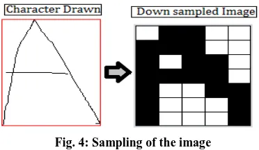
The down sampled image is considered to have dh Height and dw Width. Down-sampling [2] is necessary to produce input neurons for the neural network. The sampling procedure begins with dividing the bounded image of H height and W width into dh*dw block each of height H/dh and width W/dw. Here H/dh is the height ratio [3] and W/dw is the width ratio.
The algorithm then iterates through each of the blocks and search if there is a black pixel in the block. If there is a black pixel value, the pixel (xi,yj) of the down sampled image is marked as black else the pixel is marked as white. The height of the down sampled image is 7 pixels and width 5 pixels. Thus have dh=7 and dw=5.
[image:2.595.100.234.67.187.2]\
Fig. 4 shows the down sampled image conversion.
Fig. 4: Sampling of the image
There are 35 input neurons from the 7*5 pixels in the down sampled image as shown in Fig. 4. These 35 input neurons are used in the next step.
This completes the feature extraction process and the next process follows. The next step is Training Process for the Back Propagation Network.
3. BACK-PROPAGATION NEURAL
NETWORK TRAINING
Back-Propagation Network [3], [4] is a kind of Network used for supervised learning. The network consists of three layers. The first layer is the input layer, the second layer is the hidden layer and the third layer is the output layer.
[image:2.595.335.521.83.191.2]Fig. 5 gives the architecture of the BPN used for identifying input patterns.
Fig. 5: BPN Architecture used for Recognizing Characters Drawn
For each character in the list there are 35 input neurons as there are 7*5 pixel values in the down sampled image. The inputs can be ‘0’ or ‘1’. There can be a maximum of 26 output neurons denoting 26 English alphabets. For every input pattern only one of the 26 output patterns will be 1 representing the index in the list and the rest will be 0. Fig 5 gives the architecture of the BPN neural network. ‘0’ here denotes white pixel (pixel value ‘1’) and ‘1’ denotes a black pixel (pixel value ‘0’).
The steps for training the network is given in Fig. 6.
Fig. 6: Steps in BPN Training
The weight matrix is initialized along with other parameters. After initialization, the following step is continued up to 60000 epochs or until the max error is in the feed-forward step is less than equal to 0.005.
Thus for each pattern in the list the following loop is continued
Epoch=0
While maxError>0.005 and Epoch<=60000 For i = 0 To No. of training patterns added FeedFowrd(inpuPattern(i))
BackPropagationError() UpdateWeigt()
Epoch=Epoch+1 End Loop
[image:2.595.76.524.390.540.2]Here maxError is calculated as the absolute error produced or the maximum difference between the expected output pattern and the generated output pattern.
Table 1 gives the list of parameters used and their initial values.
Table 1: Parameters used in Training
Parameters Denoted By Initialized values
No. of input Neurons
n 35
No. of hidden layer Neurons
m 20
No. of output Neurons
k 26
Input Neurons x(i) where 0<=i<n 0 Hidden Neurons Zhid(i) where
0<=i<m
0
Output Neurons Zout(i) where 0<=i<k
0
Weights from input layer to hidden layer
V(i,j) where 0<=i<n and 0<=i<m
Random numbers between -0.5 and +0.5
Weights from hidden layer to output layer
W(i,j) where 0<=i<m and 0<=i<k
Random numbers between -0.5 and +0.5
Bias for hidden layer
hidBias(i) where 0<=i<m
Random numbers between 0 and 1 Bias for output
layer
outBias(i) where 0<=i<k
Random numbers between 0 and 1 Error information
for hidden layer
δout(i) where 0<=i<m
0
Error information for output layer
δhid(i) where 0<=i<k
0
Learning rate α 0.5
Momentum μ 0.4
Each step is described with more details.
3.1 Initialization Step
The down-sampled image has 7*5 blocks [4] and thus there are 35 input neurons considering each block as one input neuron.
The weights of the input layer to hidden layer are given random values. Similarly the weights of the hidden layer neurons to output layer neurons are assigned random values between -0.5 to +0.5.
3.2 Feed Forward
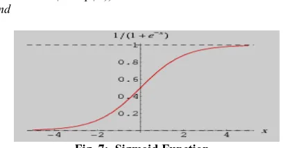
The sigmoid function is used as the threshold function for the feed-forward step. (Fig. 7)
Function thresh(x) Return 1/(1+exp(-x)) End
Fig. 7: Sigmoid Function
Every input neuron receives the input x(i) and transmits them to the hidden layer neurons [5], [6], [7]. For each hidden unit, Zhid, the hidden layer input denoted by Zhidin is calculated as give bellow:
For j=1 to m
Zhidin(j) = hidBias(j) For i=1 to n
Zhidin(j) = Zhidin(j) + x(i)*V(i,j) End Loop
End Loop
The output of each hidden layer unit is calculated by using the following loop.
For i=1 to m
Zhid(i) = thresh(Zhidin(i)) End Loop
The hidden layer output is transmitted to the output layer. For each output layer neurons Zout, the input to the neurons denoted by Zoutin is calculated as
For j=1 to k
Zoutin(j) = outBias(j) For i=1 to m
Zoutin(j) = Zoutin(j) + Zhid(i)*W(i,j) End Loop
End Loop
The output of each output layer unit is calculated by using the following loop.
For i=1 to k
Zout(i) = thresh(Zoutin(i)) End Loop
After the feed-forward step ends, the back propagation step for finding the errors starts. The next step is used to get the errors in the feed-forward step.
.
3.3. Back Propagation of Error
In this step the error in the previous step is calculated and that error is used to train the network again [8]. The error of the output layer is calculated first and then the hidden layer error is calculated. The error information term is denoted asδout for output layer errors and δhid for hidden layer errors which are calculated using the following delta rules. The error information for the output layer is calculated as follows
For i = 1 to k
δout(i) = (actual(i)-Zout(i)) * thresh(Zoutin(i)) * (1-thresh(Zoutin(i))
End Loop
Similarly the error information for the hidden layer is calculated as follows
For i = 1 to m temp=0 For j=1 to k
temp=temp+ δout(i)*W(i,j) End Loop
[image:3.595.50.291.150.459.2] [image:3.595.61.265.648.755.2]After the completion of this step the errors of the Feed-forward steps are calculated.
3.4. Weight Update
In this step the errors calculated in the previous step are used to update the weights before the next epoch begins. The weights are updated as follows [9], [10], [11].
Initially the weights of the hidden to output layer are updated.
For i = 1 to m For j = 1 to n
W(j,i,)t+1 = W(j,i)t + α*δout(i)*Zhid(j) +
μ*(W(j,i)t - W(j,i)t-1) End Loop
End Loop
In the above loop α*δout(i)*Zhid(j) is the weight correction term denoted by ΔW(j,i) .
The output of each hidden layer unit is calculated by using the following loop.
For i=1 to m
Zhid(i) = thresh(Zhidin(i)) End Loop
The bias of the output layer units are updated as follows
For i = 1 to k
outBias(i)= outBias(i) + α*δout(i)
End Loop
The new weights of input layer neurons to the hidden layer neurons are now calculated.
For i = 1 to k For j = 1 to m
V(j,i,)t+1 = V(j,i)t + α*δhid(i)*x(j) +
μ*(V(j,i)t - V(j,i)t-1) End Loop
End Loop
The bias of the hidden layer units are updated as follows
For i = 1 to m
hidBias(i)= hidBias(i) + α*δhid(i)
End Loop
4. APPLYING THE NEURAL NETWORK
The neural network is trained for all the letters added to the list. For each character in the list there are 35 input neurons and 26 output neurons. For every input patter only one of the 26 output patterns will be 1 representing the index in the list and the rest will be 0.The parameters used in this algorithm are same as in the Training step [12], [13].
Every input neuron receives the input x(i) and transmits them to the hidden layer neurons.
For each hidden unit, Zhid(i), the hidden layer input Zhidin(i) is calculated as give bellow:
For j=1 to m
Zhidin(j) = hidBias(j) For i=1 to n
Zhidin(j) = Zhidin(j) + x(i)*V(i,j) End Loop
End Loop
The hidden layer output is transmitted to the output layer. For each output layer neurons Zout(i), the input to the neurons, Zoutin(i) is calculated as
For j=1 to k
Zoutin(j) = outBias(j) For i=1 to m
Zoutin(j) = Zoutin(j) + Zhid(i)*W(i,j) End Loop
End Loop
The output of each output layer unit is calculated by using the following loop.
For i=1 to k
Zout(i) = thresh(Zoutin(i)) End Loop
Only one of the 26 output neurons will be activated that represents the list index of the added alphabets.
5. IMPLEMENTATION
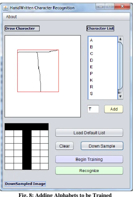
The algorithms used above are now tested and with the help of a GUI, English alphabets are added to the list. Initially some training data is added to the list by drawing characters in the user interface. After every character is added, an input pattern is generated using the Feature Extraction process. The next step which is the Training Process follows the algorithms discussed in this paper. A GUI is used for drawing characters and identifying them. Initially 10 alphabets are added. [A,B,C,D,E,P,K,R,S,T] are added as shown in Fig. 8.
[image:4.595.323.538.403.722.2]
Fig. 8: Adding Alphabets to be Trained
The training process is now started and after every epoch the error is shown in the command line window (Fig. 9). It is seen that initially the error is quite high and after every epoch it reduces and finally when it reaches a max error of 0.005 the training is completed.
Fig. 9: Training Process showing Error after every epoch
[image:5.595.319.537.101.507.2]After the training is completed, the network can be used to identify alphabets drawn in the interface.
Table 2 shows the accuracy of recognizing each character
Table 2: Accuracy of the 10 characters in the list Characters
Drawn
No. of times drawn
No. of times Recognized
Accuracy
A 10 9 90%
B 10 7 70%
C 10 10 100%
D 10 9 90%
E 10 9 90%
P 10 8 100%
K 10 7 70%
R 10 8 80%
S 10 9 90%
T 10 10 100%
[image:5.595.55.292.136.460.2]The recognition output generated by drawing a character ‘A’ is shown in Fig. 10.
Fig. 10: Recognizing character ‘A’
Table 3 gives the recognition accuracy rates after training the network for a certain number of characters.
Table 3: Results for recognizing English Alphabets No. of
Training patterns
Accuracy No of Epoch
Max Error
10 86% 11000 0.005
18 81% 37000 0.005
26 79% 60000 0.008
The above results conclude that the back propagation approach can be used for recognizing English alphabets drawn by the help of a stylus.
The same network can be used for recognizing numbers and the accuracy for using the same Network for recognizing digits are given in Table 4.
Table 4: Results for recognizing Numbers No. of
Training patterns
Accuracy No of Epoch
Max Error
[image:5.595.50.275.540.763.2]6. CONCLUSION AND FUTURE SCOPE
Using the Back-Propagation Network, characters drawn with the help of a stylus can thus be recognized. The algorithms used are shown and the results using them are given. The results of the shown back-propagation approach are acceptable for recognizing characters. The time taken for training is a factor and for large number of characters, the neural network may take some time to train itself. Other neural network models like Kohonen Network [14] also provides good results. This approach can also be extended to recognizing handwritten paper documents. For paper documents, one can initially scan the document and convert it to binary using an adaptive threshold and then segment the lines and then find words. From the words one can find character outlines and use the back-propagation approach to identify the characters. The network can also be trained with multiple languages so that it can be used to recognize multiple languages by using different dataset for different languages.7. REFERENCES
[1] C. Bahlmann. Directional features in online handwriting recognition. Pattern Recognition, 39(1):115–125, 2006.
[2] Anil.K.Jain and Torfinn Taxt, “Feature extraction methods for character recognition-A Survey,” Pattern Recognition, vol. 29, no. 4, pp. 641-662, 1996.
[3] Jeff Heaton, Introduction to Neural Networks with Java, Heaton Research
[4] Ernest Istook, Tony Martinez, IMPROVED BACKPROPAGATION LEARNING IN NEURAL NETWORKS WITH WINDOWED MOMENTUM, International Journal of Neural Systems, vol. 12
[5] Vu N.P. Dao 1, Rao Vemuri, A Performance Comparison of Different Back Propagation Neural Networks Methods in Computer Network Intrusion Detection
[6] Magoulas, G.D., Androulakis, G. S., and Vrahatis, M.N., Improving the Convergence of the Backpropagation Algorithm Using Learning Rate Adaptation Methods., in Neural Computation, Vol. 11,MIT Press.
[7] Davis, R.H., Lyall, "Recognition of hand written character, A review", Image and vision computing, 1986
[8] R.G. Casey and E.Lecolinet, “A Survey of Methods and Strategies in Character Segmentation,” IEEE Transactions on Pattern Analysis and Machine Intelligence, Vol. 18, No.7, July 1996
[9] C. L. Liu, H. Fujisawa, “Classification and Learning for Character Recognition: Comparison of Methods and Remaining Problems”, Int. Workshop on Neural Networks and Learning in Document Analysis and Recognition, Seoul, 2005.
[10] F. Bortolozzi, A. S. Brito, Luiz S. Oliveira and M. Morita, “Recent Advances in Handwritten Recognition”, Document Analysis, Umapada Pal, Swapan K. Parui, Bidyut B. Chaudhuri, pp 1-30.
[11]
J.Pradeep1, E.Srinivasan2, S.Himavath, "DIAGONAL
BASED FEATURE EXTRACTION FOR
HANDWRITTEN ALPHABETS RECOGNITION
SYSTEM USING NEURAL NETWORK" , IJCSIT, Vol 3, No 1m Feb 2011
[12] Anita Pal & Dayashankar Singh, “Handwritten English Character Recognition Using Neural Network”, Network International Journal of Computer Science & Communication.vol. 1, No. 2, July-December 2010
[13] N. Arica and F. Yarman-Vural, “An Overview of Character Recognition Focused on Off-line Handwriting”, IEEE Transactions on Systems, Man, and Cybernetics, Part C: Applications and Reviews, 2001