Power Grounding Optimization

http://dx.doi.org/10.4236/ajcm.2015.53021

Power Grounding Optimization

Eduardo A. Cano-Plata, Oscar J. Soto-Marín, Guillermo Jiménez-Lozano, Jorge H. Estrada-Estrada

Departamento de Ingeniería Eléctrica, Electrónica y Computación, Universidad Nacional de Colombia, Manizales, Colombia

Email: [email protected]

Received 9 June 2015; accepted 22 August 2015; published 26 August 2015

Copyright © 2015 by authors and Scientific Research Publishing Inc.

This work is licensed under the Creative Commons Attribution International License (CC BY). http://creativecommons.org/licenses/by/4.0/

Abstract

In this paper we discuss the finite element models (FEM) using electromagnetic theory—Maxwell’s equations. Next we developed a new procedure for optimization with the idea to be implemented in the standard IEEE-80 (2013). We expose those ideas in the paper. ETAP program and Matlab software are used for FEM.

Keywords

Finite Element Method, Grounding Systems, Circuit Model, ETAP Model, Engineering Design

1. Introduction

The protective scheme design is an important aspect in design and construction of the substations. The voltage gradients are created across ground mesh and points linked to earth as references [1]-[3]. The difference in po-tential is kept within the limits provided by IEEE Standards Documents and should be continuously monitored for the equipment’s proper functionality and people safety working in surrounding.

The followings are design parameters and control that define the construction of grounding system: ground potential rise (GPR), step voltage (Vstep), touch voltage (Vtouch), ground resistance (Rg), mesh voltage (Vmesh) and grid current (Ig). There are various methods available for designing of ground mesh for substation; IEEE 80- 2013 and Finite Element Method (FEM) [4] [5] are adopted for design of ground system in research conducted as these are more reliable ones.

2. Representation of the Continuity Equation

The abstracted definition of the finite element is following: the triple ordained A Bk, k,Ωk it can be represented by Ak the set of degree of freedom (nodes) it is a base of a space that genera the function Bk, it is normally a con-stitutive relation, and the domain Ωk the geometrical space.

A construction of the finite element is related to the Lagrangian method and it possible to make identifying any equilibrium configuration. In this case the so-called Updated Lagrangian formulations, plus finding the spa-tial configuration corresponding to an instant t. An instant is a given value in a temporal coordinate. The notion of time here is used in a general sense; such as a coordinate that serves to number events.

The spatial configuration corresponding to the instant t is defined by tJ current densities that satisfy the Max-well continuity equation of type [6]:

( )

0, t t t

J E σ J

∇ ⋅ = = ∀ Ω (1)

where

, ,

x y z

 ∂ ∂ ∂ 

∇ = _{∂ ∂ ∂} 

  (2) The second order tensors tσ are complicated nonlinear functions of tJ and of the history of the conductivity change process. A fundamental difficulty in solving Equation (1) is that the domain over which the equations must be solved is part of the solution of the problem. In essence the relationship between the constitutive Equa-tion (1), the space Ω and the dynamic of any point x in the space that satisfies the constitutive relationship is name the node of the finite element.

The mathematical problem is completed with boundary conditions at tσ and tJ, and it is solved using defined magnitudes over a reference configuration (in a sense, representation of the defined magnitudes in the spatial configuration) and solving a problem similar to the one described by Equation (1) over 0Ω (where the supra in-dex “0” indicates the adopted reference configuration).

The Green’s conductivity tensor and the second tensor of the Kirchhoff electric field are examples of defined magnitudes over the reference configuration to solve over 0Ω the nonlinear problems in the medium. This me-thodology has migrated from the techniques in mechanics of the continuous medium (computational mechanics) [7].

Simo et al. [7]-[9] describe methods used in the calculation of differentiable manifold [10] to systematize the task of finding representations over 0Ω of tensors defined in tΩ and also to systematize the formulation of ma-thematical problems defined over 0Ω equivalent to Equation (1). Although Maxwell developed equations in compact form, numerical methods should be used to solve them [11].

Modern developments of the finite element method applied to nonlinear problems of solid mechanics make rigorous use of these techniques [12]-[15]. The method discussed in this paper is used in electromagnetism to measure soil resistivity.

The aim of this work is to develop a geometric view of several calculation techniques of differentiable mani-fold such as pull-back and push-forward [16] to simply propose them as tools for engineers working on solving nonlinear problems in Continuum Mechanics using finite elements. The changes undergone by the soil in the presence of lightning must always be taken into consideration.

3. Constitutive Relations of Maxwell’s Equations

Engineering is based on the relationship that it can have the characteristics of the materials assuming always two conservation principles are met. The first is the principle of conservation of charge and the second the principle of conservation of energy. The approach of these principles can be differential or integral form (Eulerian and Lagrangian formulation).

Assume that you have a problem which only the variable representing the electric field is considered, we can then establish the constitutive relation:

( )

t t t

space invertible of the symmetrical space. It is important to highlight that tσ depends on the reference configura-tion. In this sense and since only the electrical characteristic are studied, it is understood that the principle of equipresence is respected and that no time is considered phenomenological factors of the quantum mechanics.

For studying the objectivity of the formulation, it was considered in the spatial configuration two coordinate systems, one stationary (x) and other moving (X*), since the current density tensor is a objective special tensor can be displayed as:

( )

( )

t t

J=Q t ⋅ J ⋅Q t (4)

where Q is an orthogonal tensor. Since the electric field is a objective tensor

( )

0 0

t t

E=Q t ⋅ E (5)

Since Q is valid for any orthogonal relationship, It will also be valid for the polar decomposition, i.e.:

( )

* *

0 t

t t

J = σ E (6) Or what it is the same tσ presents the principle dictates that the material is not affected by the change of coordinates or reference. The material is represented by the conductivity.

4. Conductivity

Conductivity defines the energy dissipated in instant t per unit of mass, which is associated with the dissipation of electrical current in the soil. This study mainly deals with equations of a continuous medium (1). These equa-tions in a grounding system might be represented as:

( )

, 0

t t t

a

J E J

E E en g J en

σ

Γ Ω

∇ ⋅ = = ∀ Ω

= Γ ⋅ = Γ (7)

In (7), Ω is the ground, σ is its conductivity tensor, ΓΩ is the ground surface, ga is the covariant vector in ge-neralized coordinates and Γ is the electrodes surface. The appropriate solution is the distribution of potential or the setting of potential at an arbitrary point. The dynamics must be evaluated once the grounding system ac-quires φΓ potential (system overvoltage) and Equation (8) is calculated p.u.

, d , _eq

J I J R

I

ϕ

σϕ Γ

Γ

Γ

= =

_∫∫

In practice, the ground is considered isotropic, thereby σ is replaced by a scalar (St. IEEE 80) [1]-[3].

In an assumed horizontal ground surface, the Dirichlet boundary condition Δφ = 0 is shown in Ω. The condi-tions expressed in (7) are obtained while searching for regulation. Applying to (7) Green’s identity [10]:

( ) ( )

, d ,

4 ε k x J x

ϕ ε ε

σ ∈Γ

= Γ ∈ Ω

Π

∫∫

With weak nucleus:

( )

_{( )}

₍

₎

( )

, , ,

, ,

k x r x x

r x r x

ε ε ε

ε ε

 

=_ + _′ _ = −

  (10)

The functional of the problem is expressed in (5). Discretizing gives:

( )

( )

J J N α

α

ε ε

+ =

=

∑

_

Matlab Toolbox Partial differential equations (PDE) are used in two mesh dimensions of triangular elements [17].

In summary, the solution of Equation (1) will go through:

re-lation, and the demine Ωk the geometrical space.

 Attaining the reference configuration of Equation (1).

 Solving the reference configuration representation over 0Ω thus obtaining current and conductivity density measurements.

 Obtaining conductivity tensors and current density from the reference configuration.

 Proposing the functional of the constitutive equation which might be formulated by the Galerkin technique using the minimal residual method.

 Solving using a triangular mesh seed.

In this way the proposed technique is oriented to see the potential distribution in the Ωk the geometrical space, the principal restriction in the design procedures of the standard IEEE-80 [1].

5. Practical Example

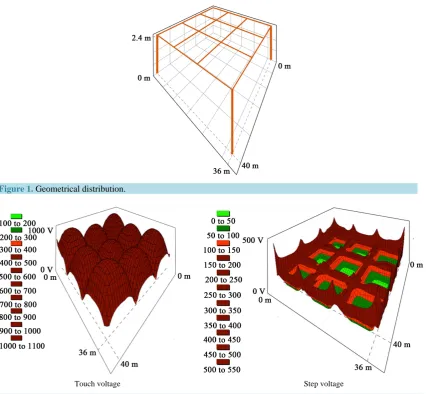
In the Table 1 its resume the parameter for one grid that is showed in the Figure 1.

The Table 1, ρ and ρS are the resistivity of the soil and surface respectively, hS and h is the deep of the grid in the soil and electrodes longitude, I0 is the fault current of the system, tC is the time protection action, and finally the L1, L2 and LV are the dimension of the grid. Figure 1shows the configuration of the mesh of the grounding system implemented in the software ETAP [18]. An example, it can be seen in [19].

The graphs for step and touch voltage are given inFigure 2.

Figure 1.Geometrical distribution.

Touch voltage Step voltage

Table 1.Physical parameters.

Parameter Value Parameter Value Parameter Value Parameter Value Parameter Value

ρS 5500 Ω⋅m tC 0.5 s h 0.5 m L2 36 m I0 10,000 A

ρ 459.2 Ω⋅m L1 40 m hS 0.2 m LV 2.4 m Grid 13.33 × 12 m2

The program provides the information below after analyzing the ground resistance information taken from the measurements of the electrical plant.

The solution using finite element analysis, for an element with three nodes, in a distribution matrix whit 320 elements and one grid from 1200 nodes.

From the finite element solution, it is possible obtained the parameter listed below it is showed in the Figure 2: Threshold levels of touch potential:

Elevation of ground potential: 4837 volts; Maximum step voltage: 7650.93 volts.

6. Comparison of Results

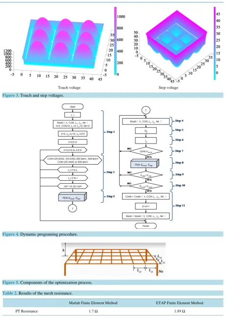
The results obtained in ETAP are compared with the method discussed in the previous section this technique was developed using MATLAB [17], the step and touch voltages are given inFigure 3.

The Table 2shows the comparison of results of the ground mesh resistance.

Table 2 shows that the results obtained are very similar which leads to the conclusion that the methods are suitable for the design and analysis of ground meshes.

This solution is so important due the necessary algorithm implementation in the optimization procedures.

7. Dynamic Optimization of IEEE-80 Procedure

The block diagram of Figure 4 illustrates the sequences of steps to design the ground grid procedure from IEEE80-2013 [1]. The parameters shown in the block diagram are identified in the index presented in Table 12 of that reference [1]. The principal parameter for that block diagram is GPR, Estep and Etouch Step 7, 9 and 10 re-spectively. We changed the step 8 it was introduced the Finite Element Method to calculate the Emesh and Etouch. They are the restriction of the dynamic programming approach. They can be obtained using the method de-scribed in the previous section.

As it is showed for the Figure 3, the tradition for the use of the design of power systems grid is the Dynamic programing that is so close to the dynamic optimization. The tradition by Richard Bellman’s method [20]. It is to model and interpolated the behavior of model under assumption of forward looking optimizing behavior. Dy-namic optimization deals with the problem of obtaining a sequence of optimal choices under given dyDy-namic constraints. Dynamic programing is the most commonly used technique this part of the paper we are working to show a computational implementation given its recursive structure it is make in the step 11, that is an important modification to the diagram block in IEEE-80 it is showed in theFigure 3.

Description of the Optimization Problem

The grounding grid is composed for linear conductors. Each conductor is subdivided in small linear segments. We can obtain the current density in each segment using the complex images method [3]. Figure 5 shows the grounding grid.

The objective function is described by.

(

)

( )

(

)

, , , ,

min _{x x y y k k i j}

x y k i j

L CL L CL Ne CNe h CON

 

+ + + +

 



∑

Constrains:

touch touch _ min

step step _ min

Touch voltage Step voltage

Figure 3. Touch and step voltages.

Figure 4. Dynamic programing procedure.

Figure 5. Components of the optimization process.

Table 2.Results of the mesh resistance.

Matlab Finite Element Method ETAP Finite Element Method

where:

ne: number of electrodes;

CNe: is the total cost of electrodes including the installation; Lx: number of horizontal electrodes in the direction X,

CLx: is the total cost of the electrodes including the installation; Ly: number of horizontal electrodes in the direction Y;

CLy: is the total cost of the electrodes including the installation; h: is the deep respect to the surface of the grid;

CON: is the cost of the conductor diameter; A: area.

The Table 3 shows the parameter of the Equation (12).

To solve the problem, the dynamic programming approach uses a recursive method that works backwards. For the Equation (10) the method work as follows:

 Compute the cost J of each component in the each grid configuration (in the last stage).

 Compute the cost of each feasible optimal sequence of component for the each node which implies the op-timal sequence to the construction of the grid if opop-timal sequence problem.

 Its solved is optimal it ask to the constriction step 9, 10 and 12 of the flow, the Figure 4.

It is very similar to the economic application in which a structured proposed grid with the voltage as a state variable is evolves troughs time. This system can be manipulated by means of a set or blocks of construction part of the grid (electrodes and cables) in order to minimize the cost function (10).

Remember that the dynamic programming approached works by solving the problem backward in time, de-termining the optimal grid, it is transform the original (10) problem and an subsequence of sub-problems. It is a crucial notion of the cost-to-go, which is the cost along minimum-cost path from a given grid stated.

The general approach:

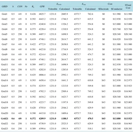
Figure 6 shows the configuration of the grounding system optimal. The Table 4 is the result from application of this algorithm to the optimal design problem in an 115 kV substation and therefore the grounding system op-timal is the number 21 (Grid21) of the table.

Table 3.Parameters used in the Equation (12).

Element Cost

Ne $35.00

CON 4/0 AWG $12.50

CON 250 kcmil $45.00

Installation cost (m2_{) $7.00}

Figure 6.Optimal ground system.

Table 4. Results of the optimization process.

GRID h CON Ne Rg GPR

Etouch Estep Cost _$Total

Cost Tolerable Calculated Tolerable Calculated $Electrode $Conductor

Grid1 0.5 4/0 0 0.426 4825.7 1231.0 2685.9 4373.7 762.6 $0 $11.980 $11.980

Grid2 0.5 4/0 0 0.392 4443.2 1231.0 1746.5 4373.7 615.5 $0 $12.930 $12.930

Grid3 0.5 4/0 0 0.375 4240.8 1231.0 1326.2 4373.7 554.8 $0 $13.880 $13.880

Grid4 0.5 250 0 0.373 4228.4 1231.0 1310.9 4373.7 554.8 $0 $23.760 $23.760

Grid5 0.5 250 0 0.389 4407.3 1231.0 1698.9 4373.7 524.3 $0 $20.340 $20.340

Grid6 0.5 250 0 0.419 4748.1 1231.0 2614.7 4373.7 641.2 $0 $16.920 $16.920

Grid7 0.6 4/0 0 0.422 4772.9 1231.0 2638.0 4373.7 641.2 $0 $11.980 $11.980

Grid8 0.6 4/0 0 0.391 4423.8 1231.0 1716.9 4373.7 524.3 $0 $12.930 $12.930

Grid9 0.6 4/0 0 0.372 4214.4 1231.0 1298.3 4373.7 474.7 $0 $13.880 $13.880

Grid10 0.6 4/0 0 0.419 4748.1 1231.0 2614.7 4373.7 641.2 $0 $11.980 $11.980

Grid11 0.6 4/0 0 0.389 4407.3 1231.0 1698.9 4373.7 524.3 $0 $12.930 $12.930

Grid12 0.6 250 0 0.371 4202.0 1231.0 1283.0 4373.7 474.7 $0 $23.760 $23.760

Grid13 0.5 4/0 1 0.425 4806.4 1231.0 2592.1 4373.7 749.2 $43 $11.980 $12.023

Grid14 0.5 4/0 1 0.393 4450.4 1231.0 1641.3 4373.7 610.8 $43 $12.930 $12.973

Grid15 0.5 4/0 1 0.374 4235.9 1231.0 1213.0 4373.7 549.8 $43 $13.880 $13.923

Grid16 0.5 250 1 0.422 4782.3 1231.0 2569.4 4373.7 749.2 $43 $16.920 $16.963

Grid17 0.5 250 1 0.392 4434.2 1231.0 1623.7 4373.7 610.8 $43 $20.340 $20.383

Grid18 0.5 250 1 0.373 4223.7 1231.0 1197.9 4373.7 549.8 $43 $23.760 $23.803

Grid19 0.6 4/0 1 0.420 4755.0 1231.0 2546.2 4373.7 629.9 $43 $11.980 $12.023

Grid20 0.6 4/0 1 0.390 4415.8 1231.0 1609.6 4373.7 518.1 $43 $12.930 $12.973

Grid21 0.6 4/0 1 0.372 4209.9 1231.0 1188.5 4373.7 470.5 $43 $13.880 $13.923

Grid22 0.6 250 1 0.418 4730.9 1231.0 2523.5 4373.7 629.9 $43 $16.920 $16.963

Continued

Grid24 0.6 250 1 0.371 4197.7 1231.0 1173.3 4373.7 470.5 $43 $23.760 $23.803

Grid25 0.5 4/0 2 0.374 4230.9 1231.0 1198.0 4373.7 545.0 $86 $13.880 $13.966

Grid26 0.5 4/0 2 0.392 4441.5 1231.0 1614.5 4373.7 603.7 $86 $12.930 $13.016

Grid27 0.5 4/0 2 0.422 4776.7 1231.0 2495.7 4373.7 729.4 $86 $11.980 $12.066

Grid28 0.5 250 2 0.421 4763.2 1231.0 2507.5 4373.7 736.2 $86 $16.920 $17.006

Grid29 0.5 250 2 0.391 4425.5 1231.0 1597.1 4373.7 603.7 $86 $20.340 $20.426

Grid30 0.5 250 2 0.373 4218.8 1231.0 1183.1 4373.7 545.0 $86 $23.760 $23.846

Grid31 0.6 4/0 2 0.418 4736.7 1231.0 2484.9 4373.7 619.0 $86 $11.980 $12.066

Grid32 0.6 4/0 2 0.389 4407.6 1231.0 1583.3 4373.7 512.1 $86 $12.930 $13.016

Grid33 0.6 4/0 2 0.371 4205.2 1231.0 1173.8 4373.7 466.4 $86 $13.880 $13.966

Grid34 0.6 250 2 0.416 4713.2 1231.0 2462.7 4373.7 619.0 $86 $16.920 $17.006

Grid35 0.6 250 2 0.388 4391.6 1231.0 1565.9 4373.7 512.1 $86 $20.340 $20.426

Grid36 0.6 250 2 0.370 4193.1 1231.0 1150.8 4373.7 464.2 $86 $23.760 $23.846

Grid37 0.5 4/0 3 0.421 4766.9 1231.0 2470.2 4373.7 723.8 $129 $11.980 $12.109

Grid38 0.5 4/0 3 0.391 4432.4 1231.0 1588.6 4373.7 596.7 $129 $12.930 $13.059

Grid39 0.5 4/0 3 0.373 4225.7 1231.0 1183.4 4373.7 540.3 $129 $13.880 $14.009

Grid40 0.5 250 3 0.419 4743.9 1231.0 2448.5 4373.7 723.7 $129 $16.920 $17.049

Grid41 0.5 250 3 0.401 4541.8 1231.0 1585.0 4373.7 611.2 $129 $20.340 $20.469

Grid42 0.5 250 3 0.372 4213.8 1231.0 1168.7 4373.7 540.3 $129 $23.760 $23.889

Grid43 0.6 4/0 3 0.417 4718.2 1231.0 2426.4 4373.7 608.5 $129 $11.980 $12.109

Grid44 0.6 4/0 3 0.389 4399.2 1231.0 1557.9 4373.7 506.2 $129 $12.930 $13.059

Grid45 0.6 4/0 3 0.371 4200.4 1231.0 1159.5 4373.7 462.3 $129 $13.880 $14.009

Grid46 0.6 250 3 0.415 4695.3 1231.0 2404.7 4373.7 608.5 $129 $16.920 $17.049

Grid47 0.6 250 3 0.387 4383.5 1231.0 1540.7 4373.7 506.2 $129 $20.340 $20.469

Grid48 0.6 250 3 0.4 4188.5 1231.0 1144.7 4373.7 462.3 $129 $23.760 $23.889

8. Conclusion

In the present paper we discussed the application of the finite element method and dynamic programing to the design of the ground power systems (electrodes and mesh ground). Considering that these procedures are nor-mally used in other areas, it is very important to introduce physical knowledge as much as possible, in order to “guide” the solution in the case of IEEE 80-2013 standard application in the particular case of Electrical Engi-neering work.

References

[1] ANSI/IEEE Standard 80-2013 Guide for Safety in AC Substations Grounding.

[2] Practical Applications of ANSI/IEEE Standard 80-1986—IEEE Guide for Safety. Garret, D.L Org., 86 EhO253-S-PWR. [3] Casas Ospina, F. (2010) Grounding—Safety in Power Systems (Spanish). INCONTEC, 187p,

[4] Zienkiewicz, O.C., Taylor, R.L. and Zhu, J.Z. (2005) The Finite Element Method. 6th Edition, Elsevier, Barcelona. [5] Reddy, J.N. (2005) An Introduction to the Finite Element Method. McGraw-Hill, New York.

FEM (Spanish). National University of Colombia, Manizales.

[7] Simo, J.C. (1988) A Framework for Finite Strain Elasto-Plasticity Based on Maximum Plastic Dissipation and the Multiplicative Decomposition, Part I: Continuum Formulation. Computer Methods in Applied Mechanics and Engi-neering, 66, 199-219. http://dx.doi.org/10.1016/0045-7825(88)90076-X

[8] Simo, J.C. (1988) A Framework for Finite Strain Elasto-Plasticity Based on Maximum Plastic Dissipation and the Multiplicative Decomposition, Part II: Computational Aspects. Computer Methods in Applied Mechanics and Engi-neering, 68, 199-219. http://dx.doi.org/10.1016/0045-7825(88)90076-X

[9] Simo, J.C. and Marsden, J.E. (1984) On the Rotated Stress Tensor and the Material Version of the Doyle-Ericksen Formula. Archive for Rational Mechanics and Analysis, 86, 213-231. http://dx.doi.org/10.1007/BF00281556

[10] Michiel, H. (2001) Differentiable Manifold. Encyclopedia of Mathematics. Springer, Berlin.

[11] Monk, P. (2003) Finite Element Methods for Maxwell’s Equations, Numerical Mathematics and Scientific Computa-tion. Clarendon Press, Oxford, 450.

[12] Anand, L. (1979) On Hencky’s Approximate Strain-Energy Function for Moderate Deformation. Journal of Applied Mechanics, 46, 78-82. http://dx.doi.org/10.1115/1.3424532

[13] Rolph III, W.D. and Bathe, K.J. (1984) On a Large Strain Finite Element Formulation for Elasto-Plastic Analysis. In: William, K.J., Ed., Constitutive Equations: Macro and Computational Aspects, Winter Annual Meeting, ASME, New York, 131-147.

[14] Weber, G. and Anand, L. (1990) Finite Deformation Constitutive Equation and a Time Integration Procedure for Iso-tropic, Hyperelastic-Viscoplastic Solids. Computer Methods in Applied Mechanics and Engineering, 79, 173-202. (1990). http://dx.doi.org/10.1016/0045-7825(90)90131-5

[15] Eterovic, A.L. and Bathe, K.J. (1990) A Hyperelastic Based Large Strain Elasto-Plastic Constitutive Formulation with Combined Isotropic Kinematic Hardening Using the Logarithmic Stress and Strain Measures. International Journal for Numerical Methods in Engineering, 30, 1099-1114. http://dx.doi.org/10.1002/nme.1620300602

[16] Dvorki, E. and Goldschmit, M. (2002) Finite Element Method, Graduate Course. Universidad de Buenos Aires, Buenos Aires.

[17] Matlab Partial Differential Equation (PDE) Toolbox, MATLAB 7.0, 2008.

[18] ETAP 114C Power System Engineering, Operation Software Technology, 2014—Grounding Module.

[19] Soto Marin, O.J. (2015) Failure Analysis of Distribution Transformers in the East Zone of Caldas. National University of Colombia, Manizales.