Estimating Dynamic Model Parameters for Adaptive
Protection and Control in Power System
M. A. M. Ariff
, Student Member, IEEE
, B. C. Pal
, Fellow, IEEE
, and A. K. Singh
, Student Member, IEEE
Abstract—This paper presents a new approach in estimating im-portant parameters of power system transient stability model such as inertia constant and direct axis transient reactance in real time. It uses a variation of unscented Kalman filter (UKF) on the phasor measurement unit (PMU) data. The accurate estimation of these parameters is very important for assessing the stability and tuning the adaptive protection system on power swing relays. The effectiveness of the method is demonstrated in a simulated data from 16-machine 68-bus system model. The paper also presents the performance comparison between the UKF and EKF method in estimating the parameters. The robustness of method is further validated in the presence of noise that is likely to be in the PMU data in reality.
Index Terms—Measurement-based, parameters estimation, phasor measurement units, power system dynamic model, syn-chrophasors, unscented Kalman filter.
NOMENCLATURE
Continuous and discrete state variables, respectively.
Continuous and discrete output variables, respectively.
Continuous and discrete input variables, respectively.
Continuous and discrete process noise variables, respectively.
Continuous and discrete measurement noise variables, respectively.
State update and measurement function, respectively.
Estimated mean and covariance of the state. Process and measurement noise covariance, respectively.
Augmented state variables.
Manuscript received December 23, 2013; revised May 09, 2014; accepted June 14, 2014. Date of publication July 21, 2014; date of current version Feb-ruary 17, 2015. This work was supported in part by the Ministry of Educa-tion Malaysia (MOE) and in part by the Universiti Tun Hussein Onn Malaysia (UTHM). Paper no. TPWRS-01620-2013.
The authors are with the Department of Electrical and Electronics En-gineering, Imperial College London, London SW7 2AZ, U.K. (e-mail: [email protected]; [email protected]; [email protected]).
Color versions of one or more of the figures in this paper are available online at http://ieeexplore.ieee.org.
Digital Object Identifier 10.1109/TPWRS.2014.2331317
Estimated mean and covariance of augmented state, respectively.
Parameters vector.
Time step.
Dimension of state vector.
Sigma points and predicted sigma points of state vector, respectively.
Length and associated weight of sigma points, respectively.
Weighted mean and covariance of predicted sigma points, respectively.
Sigma points of predicted measurement.
Weighted mean and covariance of sigma points of predicted measurement, respectively. Cross-correlation matrix.
Kalman gain.
Rotor angle (rad) and rotor speed (pu), respectively.
Synchronous speed (pu) and base speed (rad/s), respectively
Mechanical power (pu).
Active power (pu) and reactive power (pu), respectively.
Voltage magnitude (pu) and phase angle (rad), respectively.
Generator internal voltage (pu), transient reactance (pu) and inertia constant (s), respectively.
Pseudo input for voltage magnitude and active power , respectively.
Pseudo process noise for voltage magnitude and active power , respectively.
I. INTRODUCTION
T
ECHNICAL investigations of several recent power blackouts revealed that inadequacy of control and mal-operation of protection system led to widespread system outage. A large majority of the existing control and protection logics are engineered based on model-based simulationstudies over large number of operating scenarios. With the change in generation capacity, load demand, network capacity and configuration, the control and protection settings need to be recalculated and retuned. There is always some risk in model-based system design as in reality, the dynamic behavior of complex power network with hundreds of synchronous generators, thousands of loads and transformers can never be very closely matched through model-based simulations. The famous WECC blackout in 1996 corroborated this fact, where measured response in the period just preceding the blackouts did not match with simulated results using the planning model [1].
Amongst many others, one important suggestion was an adaptive protection, mainly correct operation of Zone 3 and out-of-step relays [2]. The setting of out-of-step relay is primarily dictated by three parameters: direct axis transient reactance , quadrature axis speed voltage and generator inertia [3]. While a larger compromises the sensitivity and speed of the relay operation, a higher and require longer operation. It is clear that for accurate and secure action of the out-of-step protection unit, these parameters need to be precise. The generators manufacturers' data can be repre-sentative. Moreover, increasing addition of power electronics interfaced renewable generations at transmission level influ-ence the apparent impedance seen by the out-of-step relay during electromechanical oscillations. All these parametric uncertainties and variations demand regular update of the relay setting to suit to prevalent operating situation. It is obvious that continuous estimation of , and are required to achieve this objective.
While the PMU technology provides high resolution time-synchronized measurements, it is necessary to have a fast parameter estimation tool that is suitable to estimate the parameters for adaptive protection and control application. In practical operating environment, the PMU measurements are influenced by transient, process and measurement noise. Existing literatures do not appear to address all these aspects comprehensively. This paper reports an algorithm which we believe addresses this issue well. Our algorithm is based on the moment-matching recursive estimation using augmented unscented Kalman filter (UKF). In order to demonstrate the accuracy of the proposed technique, we have worked on data generated from 16-machine 68-bus test system model simula-tion. The UKF method is simple, accurate, fast and robust in filtering out the effect of noise in the estimated parameters.
Section II, following this introduction, reports recent and ongoing research efforts in dynamic model parameter estima-tion. Section III elucidates the approach used to utilize UKF for dynamic model parameters estimation using PMU mea-surements. Subsequently, the proposed approach is applied to measurement data simulated from 16-machine 68-bus system models. The results obtained are analyzed and discussed in Section IV. Section V compares the performance of the pro-posed method with EKF and evaluates the performance of the proposed method in the presence of noise. In Section VI, the results obtained using proposed method is validated and compared with the actual parameters. Section VII concludes our findings.
II. STATE OF THEART
The objective of dynamic model parameters estimation is to provide an accurate representation of the dynamic behavior of the system for simulation studies. Conventionally, short-cir-cuit test on unloaded machine represented the standard mea-sure of transient performance and various commonly accepted approximations formed the basis of model parameter deriva-tion. However, due to its limitation on providing q-axis tran-sient and sub-trantran-sient constant, several alternative tests, such as enhanced sudden short circuit test, stator decrement test and standstill frequency response test have been proposed to obtain better representation of the dynamic model [4]. Although accu-rate, these approaches are not economically feasible because the generator under investigation must be offline.
Online methods have been proposed to address the pitfall of the staged test approach to identify the dynamic model parame-ters. The approaches underlying these methods are diverse, e.g., trajectory sensitivity [5], extended Kalman filter (EKF) [6], non-linear least square technique [7], Newton Raphson [8] and Euler [9]. Despite having advantages over offline methods, these tech-niques have some limitations. The methods assume the avail-ability of accurate rotor angle and speed; field voltage and cur-rent; terminal voltage and curcur-rent; and active and reactive power measurements. In practice, it is not always possible to have all these measurements time-stamped.
PMU measurements driven model parameters estimation has been proposed in the literature. The PMU provides the data across the network with time synchronous stamping. The maximum likelihood estimation (MLE) is proposed to estimate the dynamic model parameters of the system in [10]. The method requires a priori additional information of the state variable to estimate the parameters accurately. Other effort integrates hybrid dynamic simulation, trajectory sensitivity, parameter correlation analysis and minimum variance crite-rion to solve the estimation problem [11]. It is non-recursive and computationally exhaustive. Another approach, inter-area model estimation (IME), is reported in [12] and [13] to estimate the parameters. The proposed method extrapolates system impedance and inertia using the inter-area oscillation compo-nents in the voltage variables after disturbance. Besides being non-recursive, the complexity of the method increases with the number of generators in the system.
comple-mentary information as required in [14]. Besides being com-putationally expensive, iterative EKF-based prediction suffers from linearization error. The robustness and accuracy associated with EKF driven methods in [14] and [15] are not thoroughly in-vestigated. The presence of noise in measured signal influences the accuracy of the dynamic model parameter estimation tech-nique. Therefore, it is important to guarantee that the dynamic model parameter estimation technique is robust in the presence of measurement noise in the signals.
In this paper, the dynamic model parameters of synchronous generators are estimated by processing the PMU measurements using unscented Kalman filter (UKF); a moment-matching filter that is significantly better than EKF. The UKF is developed to address the issues in EKF. It calculates the statistics of random variables that undergo a nonlinear transformation. This method works on the assumption that it is easier to approximate a probability distribution than it is to approximate an arbitrary nonlinear function or transformations [16]. The UKF has earlier been used in power system for dynamic state estimation [17], [18] and parameters estimation using operational data [19]. It has potential to be reformulated to solve dynamic parameters estimation problems [20]. However, the method proposed in this paper employs better sigma point distribution and filtering approach compared to [20], which reflects in a better accuracy of the parameter estimated and consumes less computing power. The UKF offers flexibility to allow information beyond mean and covariance to be incorporated in the estimations [21]. Hence, the UKF is able to estimate accurate dynamic model parameters even with the presence of noise in the measured data. Moreover, the UKF is completely data driven and recursive thus offering real opportunity of fast estimation in real time.
III. DYNAMICMODELPARAMETERESTIMATIONUSINGUKF
Generally, power system dynamics is represented using a set of continuous-time nonlinear equation, given in (1):
(1a) (1b)
where the vector represents the state variables, the vector represents the output variables, and is the input vari-ables. Equations (1) are rewritten in discrete form with a time step of , given by (2):
(2a) (2b)
The state is considered as a random variables with an esti-mated mean and an estimated covariance . The process noise in (2) is assumed to be non-additive, while the mea-surement noise is assumed to be additive. The covariance matrix for and are denoted by and , respectively. Both are assumed to be constant. Assume that (2) is parame-terized by the unknown vector . The state and the set of model parameters need to be estimated simultaneously. If is also treated as a state, then it may be augmented with to
give an augmented state vector , i.e., . The state-space model in (2) is reformulated as
(3a) (3b)
Using the same approach in (3), the process noise may also be concatenated with , resulting higher-dimensional state
random variables with an estimated mean
and covariance . Hence, the state random variable is redefined as the augmentation of the original state , the set of unknown model parameter and the process noise given in (4):
(4)
In a similar manner, the corresponding augmented state co-variance is built up from the individual coco-variance matrices of
, and given in (5):
(5)
Hence, the state-space model in (3) is rewritten as follows:
(6a) (6b)
Consequently, given that the system differential equations (DEs), the measured signals from PMU and all noise covari-ances are available, the unknown parameter vector is mated using recursive algorithm by finding the real-time esti-mates of the mean and covariance of the augmented state .
A. Unscented Kalman Filter (UKF)
The idea of UKF is the propagation of the statistical distribu-tion of state through the nonlinear equadistribu-tions. This is realized by obtaining a set of vectors called sigma points, which capture the mean and covariance of the state distribution. A set of sigma points, denoted as , are selected in such a way that the mean and covariance of these points are and . Consequently, these points are transformed into a set of transformed points by applying into a nonlinear function. This process is described as follows:
(7)
Next, the mean and covariance of the transformed points are calculated. The mean is the weighted average of the transformed points while the covariance is the weighted outer product of the transformed points. For numbers of sigma points, and are calculated as follows:
(8a)
To provide an unbiased estimate, the weight used to cal-culate and must be set such that
(9)
In this paper, for number of state, a set of points is used to distribute the sigma points. The following set of points satisfied the condition described above:
(10a)
(10b)
(10c)
(10d)
(10e)
(10f)
The set of sigma points described in (10) able to exploit any additional known information about the error distribution asso-ciated with an estimate and maintain the mean and covariance . This set of sigma points provides approximations accurate to a third order of Gaussian probability density functions, re-gardless of the forms of nonlinear transformation function used in the estimation [21]. The weight associated with the new sigma point, provides a parameter for controlling some aspect of the higher moments of the distribution of sigma points without affecting the mean of the covariance. In this paper, the value of is set such that the fourth order error for a Gaussian is min-imized [21]. Consequently, each sigma points is passed through the model of state evolution to obtain the predicted-state sigma points given as
(11)
Subsequently, the weighted mean and covariance of the pre-dicted sigma points defined as and , respectively, are calculated using (12):
(12a)
(12b)
Subsequently, the predicted sigma points are instantiated through the measurement equation to generate the predicted-measurement sigma points as follows:
(13)
Consequently, the weighted mean of the predicted measure-ment , the corresponding covariance matrix and the cross-correlation matrix are computed as shown in (14).
The matrix represents the cross-correlation between the difference of the predicted-state sigma points with the corresponding predicted-state , and the difference of pre-dicted-measurement sigma points with the corresponding predicted-measurement :
(14a)
(14b)
(14c)
Finally, the Kalman gain matrix is calculated to find the mean and covariance matrix as given in (15):
(15a)
(15b)
(15c)
B. Implementation of UKF for Dynamic Model Parameters Estimation
Power system first swing dynamics is represented as follows:
(16a)
(16b)
where , , , and are rotor angle, rotor speed, syn-chronous speed, and base speed, respectively. Neglecting the damping coefficient , the discrete form of (16) is given by
(17a)
(17b)
Since and are constant, is simplified by substi-tuting the term with to reduce the nonlinearity of the equation. Consequently, the state vector of the system given in (17) is defined as and is parameterized by in-ertia constant , transient impedance and generator internal voltage . These parameters and variable are unknown and
represented by the vector . As described
in (3), the state and the unknown parameter vector are si-multaneously estimated by augmenting these two vectors into a
higher-dimensional state variables .
Hence, to accommodate this change, the state evolution equa-tion in (17) is reformulated as
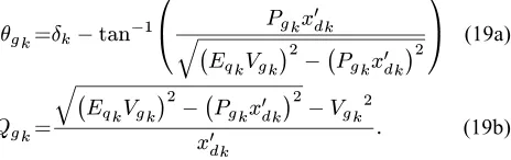
In (18), the mechanical input power is assumed to be known. It is approximated to the electrical power measured at the generator terminal bus prior to a disturbance in the system. The dynamic behavior of one generator unit can be analyzed independently from the dynamic behavior of the rest of the net-work. This is realised by separating the signals at the terminal bus into two groups: inputs and measurements. It is assumed that PMU provides time-tagged voltage magnitude , phasor angle , active power , and reactive power measurements at the generator terminal bus to monitor the dynamic behavior of the generators. Hence, and at the terminal bus are treated as the input signal, while and are treated as the measure-ment to decouple one generation unit from the rest of the system. The equations for the measurement quantities, and of a generation unit are
(19a)
(19b)
In the presence of noise in the measured signals, dealing with and may cause a problem to the UKF algorithm. Hence, the actual values of and have to be redefined to include the effect of noises in the estimation algorithm. Consequently, the actual inputs ( and ) are equal to the differences of their measured values ( and ) and the associated noises ( and ). The associated noises and also drive the system modeled in the UKF algorithm. They are modeled as in [17] and given as follows:
(20a) (20b)
Hence, and formed a pseudo input vector while and formed a pseudo process noise vector . As derived in (4), the process noise is concatenated with the state vector and the unknown parameters vector to form an augmented state . This formulation incorporates the process noises into the predicted state vector with the same level of accuracy as the propagated estimation errors without the needs to calculate the Jacobian, Hessian, or other numerical approxi-mation [16]. Therefore, the UKF algorithm as described in the preceding subsection will be directly applied to estimate .
IV. APPLICATION, RESULTS,ANDANALYSIS
[image:5.592.315.541.63.227.2]The 16-machine 68-bus system model is considered as the test system. The bus data, line data and dynamic characteris-tics of the systems are available in [22]. Fig. 1 shows the single line diagram of the system. Nonlinear simulations of the test system model are performed in MATLAB Simulink. The syn-chronous generators in the test system are modeled as classical models. The mechanical power input to the generators is as-sumed to be constant. The disturbance considered for this study is a three-phase bolted fault at bus 21. The fault is applied at and cleared by removing line 21–22 after 100 ms. The proposed method is applied on the measured data 800 ms following the clearance of the fault to avoid transient error of
[image:5.592.58.290.247.320.2]Fig. 1. 16-machine 68-bus test system model.
Fig. 2. Generator #4 measured data for 16-machine 68-bus system model.
the PMU estimation during the transition period from pre-fault to post-fault condition [2]. For parameter estimation, the pro-posed method is applied to the voltage magnitude , voltage phase angle , active power , and reactive power signals from 16 machines.
The main aim of the proposed methodology is to provide a parameter estimation tool for adaptive protection and control application, mainly for adaptive out-of-step protection. There-fore, the scope is focused on the dynamic in power swing time scale (0.5 to 0.8 Hz) [23]. In this time scale, the speed voltage is relatively constant because of large field circuit time con-stant (concon-stant flux linkage situation). Transient reactance and inertia constant will not be affected by the inclusion of sophisticated electromagnetic dynamics model. Therefore, a classical model (speed voltage behind a transient reactance) is adequate for the purpose of this investigation. The choice of sampling frequency is important. In this paper, 120 Hz was used as recommended for 60-Hz system in the recent IEEE Standard for Synchrophasor Measurements for Power System C37.118.1-2011 [24].
[image:5.592.305.551.261.452.2]Fig. 3. Genarator #4 parameters estimation for 16-machine 68-bus system model.
but not shown because of the lack of space. As described in Section III, and are used as the input, while and are used as the measurements for the UKF. The proposed method is applied to the whole set of measured data and the parameters are estimated. The initial parameters for UKF algorithm used in this paper are described as follows:
(21a) (21b) (21c) (21d)
(21e)
(21f)
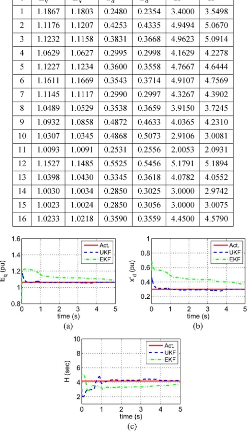
The values of initial parameters influence the convergence rate of the proposed method. The closer the value of initialised parameters with the actual value of the parameters, the faster is the convergence of the proposed method in estimating the dynamic model parameters of the system. However, the work presented in this paper assumes that the initial parameters are unknown. Therefore, the proposed method is initialised at the same value to provide an unbiased assumption in estimating the dynamic models parameters using UKF. The initial values for the covariance matrix of and are not important. It will be updated throughout the UKF iteration process and its value will become zero if the algorithm converged. On the hand, the values of and represent the process and measure-ment noise covariance matrix and their values are assumed to be known. Fig. 3 shows the results of the dynamic model parame-ters estimation for the 16-machine 68-bus test system model.
[image:6.592.310.550.63.155.2]Fig. 3(a), 3(b), and 3(c) displays the convergence of , , and , respectively. The dashed line indicates the convergence of estimated parameters obtained using the proposed method,
Fig. 4. Generator #4 state estimation for 16-machine 68-bus system model.
TABLE I
COMPARISONWITHACTUALVALUE FOR16-MACHINE68-BUSSYSTEM
while the solid line represents the actual parameters of the test system. In this application, the parameters are assumed to be un-known. The initial parameters were set arbitrarily. All the results in the figure converged to their actual value. is initialized ar-bitrarily at 1.0 pu. After first iteration, increased before it became constant at 1.1250 pu after 1.0 s. On the other hand, the initial value of is set to 0.5 pu arbitrary. After 1.0 s, is converged to 0.3868 pu. Similar observation can be made for
[image:6.592.76.293.389.525.2], where the value is initially set at 5.0 s and consequently con-verged at 4.1627 s after 1.0 s.
Fig. 4 shows the estimation of rotor angle and speed of Gen-erator #4. The dashed line indicates the estimated state, while the solid line represents the simulated state. The estimated rotor angle and speed match very well with the simulated rotor angle and speed of the machine.
proposed in this paper are accurate and consistent for all ma-chines in a large interconnected power system context.
The proposed method is able to estimate the dynamic model parameters of the systems without prior knowledge of system model. The UKF method requires a time window of 1.0 s to estimate the parameters accurately. Therefore, the method re-quires 120 iterations to precisely estimate the parameters using the measured data sampled at every 8.33 ms. The speed of com-putation of UKF method recorded in MATLAB Simulink envi-ronment is 281.2 per iteration. Hence, considering the time windows required for estimation and the computation time of UKF, it only requires 1.0337 s for the proposed method to pre-cisely estimate , , and at real time. Typically, a power swing oscillates with the frequency of 0.5–0.8 Hz [23], which gives a time windows of 1.25–2.0 s to analyze the oscillation as it develops. Thus, the speed of estimation using the proposed method is sufficiently fast for adaptive out-of-step protection application which focuses only on the first few swings of the system.
V. COMPARISON ANDPERFORMANCEROBUSTNESS
In this section, the accuracy of the dynamic model param-eters estimated using the proposed method is compared with the results obtained using the EKF approach [14], [15]. The performance of the proposed method and the EKF method is also evaluated in the presence of noise in the measured signals. Using identical operating condition, the 16-machine 68-bus test system model is used for this evaluation.
A. Parameter Estimation Using EKF
The details of the EKF method for dynamic model param-eter estimation are reported in [14] and [15] and is briefly dis-cussed here to extend the discussion of the idea presented in this paper. The EKF is formulated as a two-step prediction-cor-rection process. The prediction step is a time update using the discretized differential equations as follows:
(22a)
(22b) (22c) (22d) (22e)
The discretized differential equations in (22) predict the state and measurement variables of the next time step using the esti-mated values of the state and measurement variables of the pre-vious time step. , , and are the unknown parameters that need to be estimated. Apart from the state variables, the process also estimates priori error covariance matrix corresponding to the state variables. Consequently, the estimated measurement is calculated using the following equations:
(23a)
(23b)
Next step involves the calculation of the Kalman gain, which corrects the error of the estimated state variables based on the discrepancy between the estimated and the actual measurement. The following set of equations summarized the prediction-cor-rection process of EKF.
Prediction:
(24a) (24b)
Correction:
(24c)
(24d) (24e)
where
Using this process, the unknown parameters , , and , along with other state variables will be updated at every time step. If the EKF process converged, , , and estimation will approach their actual values.
B. Comparison
In order to evaluate the performance of the proposed method, the dynamic model parameters estimated using the proposed method is compared with the results obtained using EKF. For this evaluation, 16-machine 68-bus test system model is used to simulate the measurement of , , , and for every gen-erator sampled at 120 Hz. The disturbance considered for this evaluation is similar to the disturbance considered in Section IV. Using identical initialization of the parameters, the estimation of , , and , for Generator #4 obtained using UKF and EKF is illustrated in Fig. 5.
The results in Fig. 5 show that , , and estimated using UKF and EKF converged to its actual value of 1.0 pu, 0.5 pu, and 5.0 s, respectively. This implies that both UKF and EKF are able to estimate the dynamic model parameters in the system. However, it is observed from the results that the pro-posed method shows better performance in estimating the pa-rameters, especially for the estimation of . The EKF requires about 3.5 s while the proposed method only requires about 1.0 s to converge to its actual value of . This is because the pro-posed method has a better approximation of nonlinear process in each iteration compared to the EKF approach.
Fig. 5. Comparison of UKF and EKF estimation for Generator #4.
each iteration for both methods. The EKF algorithm requires to update the Jacobian matrix at every step of computation to esti-mate , , and . On the other hand, the UKF method does not need the calculation of the Jacobian matrix. This finding is consistent with the discussion reported in [25]. This implies that the EKF consumes more computing power compared to the pro-posed method in estimating the dynamic model parameters of the system.
C. Performance Robustness
1) Performance Under Noise: It is well known that the pres-ence of noise in the data influpres-ences the quality of any measure-ment-based method. This subsection evaluates the performance of the proposed technique in the presence of noise in the mea-sured signals. For this evaluation, the meamea-sured data illustrates in Fig. 2 is added with white Gaussian noise and the proposed technique is applied on this data to estimate , and of the generator. The presence of noise affects the quality of the PMU measurements. It is assessed by the total vector error (TVE) of the PMU measurements described as follows:
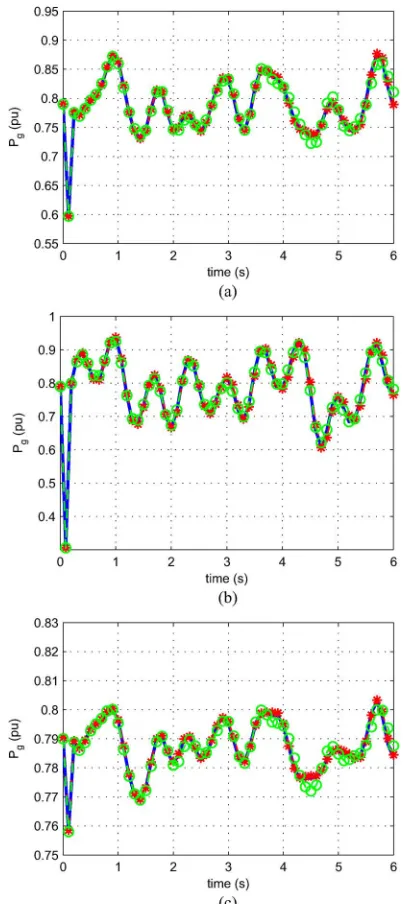
(25) As recommended in [24], the TVE of PMU measurement should be less than 1%. However, in order to validate the ro-bustness of the proposed method in filtering out the effect of noise, TVE less than 3% is used in this analysis. The plots of the data are given in Fig. 6(a)–6(d) represent , , , and for Generator #4. Fig. 7 displays the result obtained from the application of the UKF method using the measured signals with noise.
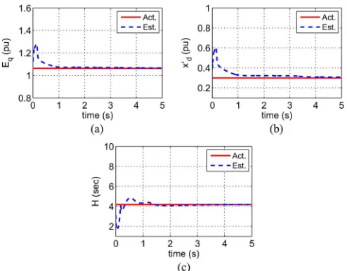
[image:8.592.305.553.63.253.2]The estimation of , , and using the measured data with noise are illustrated in Fig. 7(a)–7(c). The green lines represent the 99% confidence interval of the estimated parameters. The results clearly show that the UKF method has a fast convergence rate even with the presence of noise in the measured data. All parameters converged to the actual value in about 1.0 s. ,
Fig. 6. Generator #4 measured data with noise for 16-machine 68-bus system model.
Fig. 7. Generator #4 parameters estimation for 16-machine 68-bus system in the present of noise in measured data.
, and converged to 1.0627 pu, 0.2998 pu, and 4.2278 s, respectively. It is also observed that the actual values of the parameters lie between the upper and lower bounds for the 99% confidence interval of the estimated parameters.
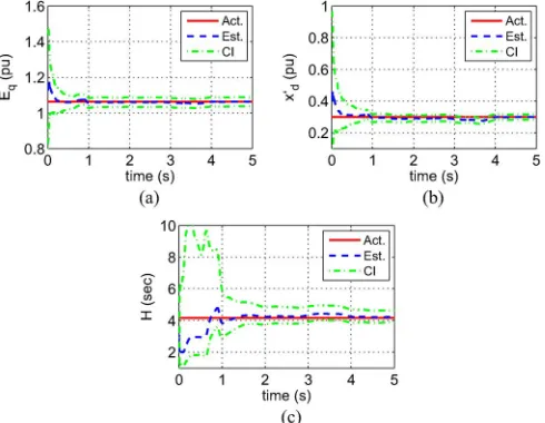
The proposed algorithm is applied to all machines in the test system model and the results are shown in Table II. In Table II, the results obtained using the UKF method is validated by com-paring the estimated results with the actual value of the dynamic model parameters. As depicted in the table, the estimated value of , , and are very close with the actual value of the dy-namic model parameters, even with the presence of noise in the measured signals.
[image:8.592.308.553.300.490.2]TABLE II
COMPARISONWITHACTUALVALUE FOR16-MACHINE68-BUS
[image:9.592.49.282.101.537.2]SYSTEMMODEL(MEASUREDDATAWITHNOISE)
Fig. 8. Comparison of UKF and EKF estimation in the presence of noise for Generator #4.
of , , and using both methods are plot in Fig. 8(a)–8(c), respectively.
The results displayed in Fig. 8 show that both methods are able to estimate accurately using the measured signals with noise. The EKF method requires about 5.0 s while the proposed method only requires about 0.2 s to estimate accurately. The estimation of and using EKF approach shows that the pres-ence of noise in the measured data influpres-ences the accuracy of the dynamic model parameter estimation technique. The EKF method shows limitation in estimating and using the mea-sured signals with noise. However, the proposed method is able to estimate and even with the presence of noise in the mea-sured data. This may be due to the fact that the approach pro-posed in this paper accurately approximate the posterior mean and covariance up to the third order of the Taylor series
ex-Fig. 9. Comparison of UKF estimation in the presence of white noise and col-ored noise for Generator #4.
pansion for any nonlinear system while the EKF method only achieved first-order accuracy [21]. The results imply that the proposed method outperforms EKF in estimating the dynamic model parameter in the system, particularly in the presence of noise in the measured data. These attributes are important for any data-driven estimation tools as the presence of the noise in measured data is inevitable.
3) Performance in Colored Noise: Colored noise covers a wide range of intensities and bandwidths for a variety of flow fluctuation during power system operation [26]. Since it may be present in the measured data, hence influencing the accuracy of any data-driven method, it is necessary to assess the opera-tion of the proposed method in the presence of colored noise in the measured signals. The colored noise used for this evaluation is generated by filtering the white Gaussian noise used to pro-duce signals in Fig. 6 through a low pass finite impulse response (FIR) filter of order 31 with normalized cut-off frequency of 0.5 [27]. The measured signals illustrated in Fig. 2 are added with the colored noise and the UKF method is applied to estimate the dynamic model parameters of the system. Fig. 9 depicts the UKF estimation trace of , , and in the presence of col-ored noise in the measured data. For the purpose of comparison, the UKF estimation in the presence of white noise is also plotted in the same figure.
From the figure, it is observed that the UKF estimation of , , and in the presence of white and colored noise demon-strate good convergence to the actual value of parameters. The performance of the proposed method in the presence of colored noise is similar to that of the proposed method in the presence of white Gaussian noise. Therefore, this implies that the proposed method is able to estimate , , and of the system in the presence of colored noise in the measured data. This is an im-portant feature for any data-driven method as the fluctuation of power flows is inevitable during power system operation.
VI. MODELVALIDATION
[image:9.592.43.288.110.534.2]re-sults obtained in Table I and II are substituted into the 16-ma-chine 68-bus test system model. Three cases with different types of disturbances were considered in this study. The disturbances considered in this analysis are as follows:
Case 1)Fault at bus 61, line 61–30 is removed to clear the fault after 50 ms;
Case 2)Fault at bus 67, line 67–68 is removed to clear the fault after 100 ms;
Case 3)Fault at bus 46, line 38–46 is removed to clear the fault after 100 ms.
Fig. 10 displays the response of the systems with this study. For all cases, the blue line indicates the response from the test system model using the actual parameters, the red line represent the response from the test system model using the actual values, and the green line represent the response from the test system model using the parameters estimated in the presence of noise in measured data. The small difference between the response of the test system models for all cases indicate that the results obtained using UKF are able to represent the dynamic response of the system, even with the presence of noise in the measured data. Thus, the dynamic model parameters estimation technique proposed in paper is accurate, consistent and robust in filtering out the effect of noise in the measured signals.
VII. CONCLUSIONS
A measurement-based dynamic model parameter estimation for power system has been proposed. The approach is based on the application of augmented UKF based technique to estimate the dynamic model parameters from wide-area voltage mag-nitude, voltage angle, real power and reactive power signals. The dynamic model parameters are estimated by augmenting the unknown states (rotor angle and speed) and parameters (in-ertia constant, transient reactance and internal voltage) into a single higher-dimensional state vector. Subsequently, the dy-namic model parameters are estimated by using the proposed UKF on the augmented state vector.
The accuracy of the estimation is validated by comparing the estimated results with the actual dynamic model parameters of the system. The presence of noise always affects the per-formance of any data driven method. Nevertheless, the UKF method accurately estimates the dynamic model parameters even with the presence of noise in the measured data. The results demonstrate that the proposed method outperforms EKF in estimating the dynamic model parameter in the system, particularly in the presence of noise in the measured data. The method is simple, fast and does not requirea prioridetails of the system information. Finally, estimating the value of the dynamic mode parameters in real time is essential to ensure appropriate operation of power system protection. This will be pursued as immediate future activity by adapting the relay characteristic to suit the current system operating condition.
ACKNOWLEDGMENT
[image:10.592.327.529.62.514.2]The authors would like to thank Dr. M. Clark for his advice and feedback on this work. The authors also would like to thank all of the anonymous reviewers for their many valuable sugges-tions that have led us to conduct additional analysis, establish deeper insight, and make well-informed conclusions.
Fig. 10. Generator #4 model validation: a) case 1; b) case 2; c) case 3.
REFERENCES
[1] P. Kundur and C. Taylor, “Blackout experiences and lessons, best prac-tices for system dynamic performance, and the role of new technolo-gies,”IEEE Task Force Rep., 2007.
[2] A. G. Phadke and J. S. Thorp, Synchronized Phasor Measurements & Their Applications. New York, NY, USA: Springer, 2008. [3] P. Kundur, Power System Stability & Control, ser. EPRI power system
engineering series. New York, NY, USA: McGraw-Hill Education, 1994.
[4] IEEE Guide for Synchronous Generator Modeling Practices and Ap-plications in Power Syst. Stability Analyses, IEEE Std. 1110-2002 (Re-vision of IEEE Std. 1110-1991), 2003, pp. 1–72.
[5] J. J. Sanchez-Gascaet al., “Trajectory sensitivity based identification of synchronous generator and excitation system parameters,”IEEE Trans. Power Syst., vol. 3, no. 4, pp. 1814–1822, Nov. 1988.
[6] B. W. Hogget al., “On-line decoupled identification of transient and sub-transient generator parameters,”IEEE Trans. Power Syst., vol. 9, no. 4, pp. 1908–1914, Nov. 1994.
[8] M. Karrari and O. P. Malik, “Identification of physical parameters of a synchronous generator from online measurements,”IEEE Trans. En-ergy Convers., vol. 19, no. 2, pp. 407–415, Jun. 2004.
[9] P. Pourbeik, “Automated parameter derivation for power plant models from system disturbance data,” inProc. 2009 IEEE Power & Energy Soc. General Meeting, Jul. 2009, pp. 1–10.
[10] D. Menget al., “An expectation-maximization method for calibrating synchronous machine models,” inProc. 2013 IEEE Power & Energy Soc. General Meeting, Jul. 2013, pp. 1–5.
[11] E. Nashawati, “PMU based generator parameter identification to im-prove the system planning and operation,” inProc. 2012 IEEE Power & Energy Soc. General Meeting, Jul. 2012, pp. 1–8.
[12] J. H. Chowet al., “Estimation of radial power system transfer path dy-namic parameters using synchronized phasor data,”IEEE Trans. Power Syst., vol. 23, no. 2, pp. 564–571, May 2008.
[13] A. Chakraborttyet al., “A measurement-based framework for dynamic equivalencing of large power systems using wide-area phasor measure-ments,”IEEE Trans. Smart Grid, vol. 2, pp. 68–81, Mar. 2011. [14] Z. Huanget al., “Generator dynamic model validation and parameter
calibration using phasor measurements at the point of connection,”
IEEE Trans. Power Syst., vol. 28, no. 2, pp. 1939–1949, May 2013. [15] L. Fan and Y. Wehbe, “Extended Kalman filtering based real-time
dy-namic state and parameter estimation using PMU data,”Elect. Power Syst. Res., vol. 103, pp. 168–177, 2013.
[16] S. J. Julier and J. K. Uhlmann, “Data fusion in nonlinear systems,” inMultisensor Data Fusion, Electrical Engineering & Applied Signal Processing Series. Boca Raton, FL, USA: CRC Press, Jun. 2001. [17] A. K. Singh and B. C. Pal, “Decentralized dynamic state estimation in
power systems using unscented transformation,”IEEE Trans. Power Syst., vol. 29, no. 2, pp. 794–804, Mar. 2014.
[18] E. Ghahremani and I. Kamwa, “Online state estimation of a syn-chronous generator using unscented Kalman Filter from phasor measurements units,”IEEE Trans. Energy Convers., vol. 26, no. 4, pp. 1099–1108, Dec. 2011.
[19] G. Valverdeet al., “Nonlinear estimation of synchronous machine pa-rameters using operating data,”IEEE Trans. Energy Convers., vol. 26, no. 3, pp. 831–839, Sep. 2011.
[20] Y. Wehbe and L. Fan, “UKF based estimation of synchronous gen-erator electromechanical parameters from phasor measurements,” in
Proc. North American Power Symp. (NAPS), 2012, Sep. 2012, pp. 1–6. [21] S. J. Julier and J. K. Uhlmann, “Unscented filtering and nonlinear
esti-mation,”Proc. IEEE, vol. 92, no. 3, pp. 401–422, Mar. 2004. [22] B. Pal and B. Chaudhuri, Robust Control in Power Systems. New
York, NY, USA: Springer, 2005.
[23] P. Anderson, Power System Protection, 1st ed. New York, NY, USA: Wiley-IEEE Press, 1999.
[24] IEEE Standard for Synchrophasor Measurements for Power Syst., IEEE Std. C37.118.1-2011 (Revision of IEEE Std. C37.118-2005), 2011, pp. 1–61.
[25] R. Kandepuet al., “Applying the unscented Kalman filter for nonlinear state estimation,”J. Process Control, vol. 18, pp. 753–768, Aug. 2008.
[26] C. Nwankpa and S. Shahidehpour, “Colored noise modelling in the reliability evaluation of electric power systems,”Appl. Math. Model., vol. 14, pp. 338–351, Jul. 1990.
[27] S. V. Vaseghi, Advanced Digital Signal Processing & Noise Reduction, 3rd ed. New York, NY, USA: Wiley, 2006.
M. A. M. Ariff(S'12) received the B.Eng degree in electrical engineering and the M.Eng degree in electrical-power from Universiti Teknologi Malaysia (UTM) in 2008 and 2010, respectively. He is pursuing the Ph.D. degree at the Department of Electrical and Electronic Engineering, Imperial College London, London, U.K.
Currently, he is a tutor in Universiti Tun Hussein Onn Malaysia (UTHM). His current research interests include of power system dynamics, coherency identi-fication, and adaptive protection in power system.
B. C. Pal(M'00–SM'02–F'13) received the B.E.E. (with honors) degree from Jadavpur University, Cal-cutta, India, the M.E. degree from the Indian Insti-tute of Science, Bangalore, India, and the Ph.D. de-gree from Imperial College London, London, U.K., in 1990, 1992, and 1999, respectively, all in electrical engineering.
Currently, he is a Professor of power systems in the Department of Electrical and Electronic Engineering, Imperial College London. His current research interests include state estimation and power system dynamics.
Prof. Pal is Editor-in-Chief of the IEEE TRANSACTIONS ONSUSTAINABLE
ENERGYand a Fellow of IEEE for his contribution to power system stability and control.
A. K. Singh(S'12) received the B.Tech. degree in electrical engineering (power) from the Indian Insti-tute of Technology, New Delhi, India, in 2010. Cur-rently, he is pursing the Ph.D. degree at Imperial Col-lege London, London, U.K.