PSO BP algorithm implementation for material surface image identification

www.arpnjournals.com

PSO-BP ALGORITHM IMPLEMENTATION FOR MATERIAL SURFACE

IMAGE IDENTIFICATION

Fathin Liyana Zainudin

_{, Abd Kadir Mahamad}

_{, Sharifah Saon}

_{, and Musli Nizam Yahya}

Embedded Computing System (EmbCoS) Research Focus Group

1_{Faculty of Electrical and Electronics Engineering, Universiti Tun Hussein Onn Malaysia, 86400 Parit Raja,}

Johor, Malaysia

2_{Faculty of Mechanical and Manufacturing Engineering, Universiti Tun Hussein Onn Malaysia, 86400 Parit}

Raja, Johor, Malaysia

ABSTRACT

Implementation of neural network for acoustic computation is not new. In this paper, a new improved method in predicting material surface from photographic image was implemented using a hybrid of particle swarm optimization and back-propagation neural network (PSO-BP) algorithm. Before the system classified the data using PSO-BP algorithm, the photographic images of room surfaces need to be extracted using Gray Level Co-occurrence Matrix (GLCM) and Modified Zernike Moments. The result indicated that the PSO-BP algorithm have a higher accuracy compared to the BP algorithm, managed to record highest accuracy of 88% as opposed to 81.3% for the latter.

Key words: Particle Swarm Optimization Back-propagation Image processing

INTRODUCTION

Material type is an important feature in room acoustic engineering; from determining the absorption coefficient of said material to computation of the room reverberation time. From the photographic images, the texture of the surfaces whether ripple, rough, smooth, etc. are captured. In analyzing the texture, the first and most important task is to extract texture features which have all the information about the textural characteristics of the original image. Previously, a few researches were performed using various types of image processing and image classification methods in building the system (Zainudin et al. 2014), (Mahamad et al. 2014), (Sari, Hazli and Shimamura, 2013). In this paper, a hybrid of particle swarm optimization and back-propagation (PSO-BP) algorithm is proposed to improve and upgrade the material surface identification system.

Application of feed forward neural network is actually a common practice for classification of the non-linearity separable patterns of the texture. Currently, there are many algorithms for feed forward neural network (FFNN) training for example the back-propagation (BP) algorithm, the Levenberg-Marquardt (LM) algorithm, the genetic algorithm (GA), and particle swarm optimization (PSO). Out of these algorithms, one of the most popular and commonly used is the BP algorithm. As it is actually a gradient based heuristic method where the concept of this algorithm is basically to search and move along the gradient towards the most minimum hence making the algorithm simple and easy to apply. The BP algorithm nevertheless had the disadvantages of slow convergence and easily getting stuck in the local minimum (Zhang et al. 2007) especially for non-linearity separable classification problems. Therefore, to overcome this particular problem, the PSO-BP algorithm is introduced to the system.

PSO algorithm itself is proven for having a fast convergence during training although it has the drawback of easily getting stuck in the global minimum (Singh and Singh,

2012). PSO-BP algorithm basically utilize PSO algorithm to find the global optimum and BP algorithm to search for the optimal weights in order to avoid getting trap in the local minimum. PSO-BP algorithm also has the upper hand of having a better convergence speed and accuracy (Han, Gu and Ju, 2011), (Liu and Qiu 2009).

PSO-BP algorithm overview

a) BP algorithm

BP architecture is not any different than any feed forward neural network where it is consists of 3 different layers; input, hidden, and output layer. The most significant difference is the existence of the back-propagation error that was feed each time to update the weights. BP algorithm neural network is still considered a supervised learning method where the desired output is needed to calculate the error that used for the weights update. The weights of BP algorithm will be updated with each iteration time. BP algorithm computes the squared error of the neural network, for gradient E as in equation (1).

𝐸 = 1

𝑁∑ |𝑡 − 𝑦|

2

(1) with N = number of training data, t = desired output and y = actual output.

The actual value of the previous expression depends on the weights of the network. BP updates the weights by shifting them along the gradient descendent direction as seen in equation (2) with η is the learning rate that controls the learning speed (Khan and Sahai, 2012).

In order to optimize, the algorithm was tested by using different numbers of hidden nodes and the one that performs best was selected. BP algorithm is fast and has high percentage of reliability but it has the disadvantage of easily getting stuck in the local minimum.

b) PSO algorithm

PSO is an algorithm that imitates the behavior of birds in a flock where each bird will continuously adjust their position and distance with one another (Ren and Yang 2010). In this algorithm, the birds are referred as particles. Each particle will fly through the search space and continuously adjust its position and velocity based on the distance between the particles own best position, pbest and the swarm best particle, gbest. In a d-dimensional search space, the position of the ith particle, xi= (xi1, xi2, xi3, …xid) is determined by

updating the velocity, v = (vi1, vi2, vi3, …vid) as in equation (3)

and updating the position as in equation (4).

𝑣𝑖𝑑(𝑡+1)= 𝑣𝑖𝑑(𝑡)+ 𝑐1𝑟1(𝑝𝑖𝑑− 𝑥𝑖𝑑(𝑡)) + 𝑐2𝑟2(𝑝𝑔𝑑− 𝑥𝑖𝑑(𝑡))

(3)

𝑥𝑖𝑑(𝑡+1)= 𝑥𝑖𝑑(𝑡)+ 𝑣𝑖𝑑(𝑡+1) (4)

where pid is the pbest position, pgd is the gbest position, c1 and

c2 are the acceleration constants or the learning factors, r1 and

r2 are vectors that sampled from a uniform distribution.

c) PSO-BP algorithm

In this hybrid algorithm, the PSO algorithm will employ the MSE from BP algorithm as its fitness measure. The following are the steps show the BP algorithm employed to the PSO algorithm.

Step 1: Initialization of PSO algorithm parameters; the position, xid, the velocity, vid, for each dimension, d.

Furthermore initialize the pbest and gbest value and compute the fitness value.

Step 2: Modify and update all the parameters; update velocity using equation (3), update position by using equation (4), update fitness value according to equation (1)

Step 3: Evaluate the parameters; if the fitness for xi is less

than fitness for pbest, then pbest=xi. If fitness for pbest less

than fitness for gbest, then gbest=pbest.

Step 4: Check whether the result meet the stop condition. If not, repeat back to step 2.

EXPERIMENTAL PROCESS

Dataset

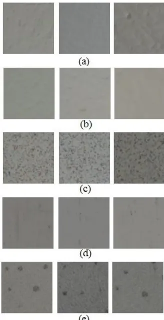
The dataset consists of photographic images of 5 different types of surface that were captured from various classrooms in Universiti Tun Hussein Onn Malaysia (UTHM). A total of 369 images were captured using a digital single-lens reflex (DSLR) camera using MICRO Nikkor 105mm 1:2.4 lens. From the total images, 90 images of the concrete wall, 93 images of the wooden wall, 60 images of the floor, 65 images of the wooden door, and 61 images of the ceiling. The distance between the camera and the surface taken for each

images were 3 feet. The respective lens setting for shutter and ISO speed were 1/50, and 400. The camera was operated using autofocus mode without using any flash. The collected image samples can be seen in Figure 1.

Figure 1: Samples of the collected material surface images; (a) concrete wall, (b) wooden wall, (c) floor, (d) wooden

door, and (e) ceiling.

All of the images in the dataset were processed using gray level co-occurrence matrix (GLCM) and modified Zernike moments.

Image Processing Implementation.

a) GLCM

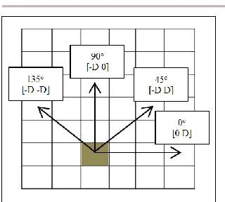
GLCM is a matrix that is build up from the spatial relationship between neighbouring pixels. The matrix can be constructed from 4 different angles, 0°, 45°, 90°, and 135°. In this experiment, GLCM were computed using distance, D=1 as well as the 4 different angles as in Figure 2 and the average value were measured.

Figure 2: Spatial relationships of pixels in an image

Using Haralick features extraction, a total of 13 textural features were extracted in this experiment. The 13 features that were computed were contrast, correlation, cluster prominence, cluster shade, dissimilarity, energy, entropy, homogeneity, autocorrelation, maximum probability, sum average, sum variance, and sum entropy. These features were used so that the textural characteristics of the images would not be lost.

b) Modified Zernike Moments

Modified Zernike Moments is a representation of an image to the Zernike polynomials, in which it is actually a series of polynomials that are orthogonal to each other (Tahmasbi, Saki and Shokouhi, 2011).

For this experiment, the photo image is transformed using Discrete Fourier Transform (DFT) and then normalized first before extracted using Zernike moments as in equation (5) where F(k1,k2) is the DFT of the image with size of N1xN2

and 0 ≤ 𝑘1< 𝑁1, 0 ≤ 𝑘2< 𝑁2, and * is the complex

conjugate. .

𝑍𝑀𝑖= |

𝑛 + 1

𝜋 ∑ ∑ log|𝐹(𝑘1, 𝑘2)|

2𝑉 ∗

𝑛𝑚(√𝜌, 𝜃)

2𝜌 𝜌𝑑𝜌

𝑘2 𝑘1

|

(5)

The magnitude for n = 1,2,3,4,5,6,7,8,9, and 10 were computed and thus bring to a total of 32 different combinations of order and repetition. For a better retrieval result for geometrically transformed textures, the mean, P0

and AC power, PAC features were also included with f(n1,n2)

is the image with size of N1xN2.

𝑃0=

∑𝑛₁∑𝑛₂𝑓(𝑛1, 𝑛2)

𝑁1𝑁2

(6)

𝑃𝐴𝐶 =

∑𝑛1∑ (𝑓(𝑛𝑛2 1, 𝑛2) − 𝑃0)2

𝑁1𝑁2

(7)

Experimental Overview

The experiments were conducted in 2 stages. The first stage is for data training and the second stage is data testing. Figure 3 shows the experimental flow that was conducted in the training stage. First, the dataset that consists of the digital images of the material surfaces were extracted using GLCM as well as Modified Zernike Moments to transform the images to its related and significant features.

The extracted data were then normalized in order to refined the dataset and eliminate redundancy of data. The normalization process will bring all data to values in the range of 0 to 1.

The normalized dataset was randomized and then divided into 3 parts. 60% of the data used for training, another 20% used for validation, and the rest 20% used for testing. In the training stage or sometimes known as the learning stage, the training dataset was trained using the PSO-BP algorithm to search for the optimal weights to fit the parameters of the classification. Both PSO and BP algorithm will work in union where the PSO algorithm will move towards the MSE in the BP algorithm. The BP algorithm simultaneously will update the particle’s position of the PSO algorithm.

Figure 3: Material surface identification system with implemented of PSO-BP algorithm in the training stage.

The validation dataset were applied in the training stage as a mark to indicate the stopping point for the algorithm before it becomes too familiar with the training dataset. Hence, validation process is important to avoid over-fitting occurrence.

The final weights were then used in the final system as constant after training is finished. The next step is to test the final system to determine the system accuracy and reliability.

yes no

Photographic images

Image extraction

Final weights PSO

algorithm

BP algorithm

MSE validation increases from previous epoch?

The main purpose of the testing stage is to assessed the performance of the system. The testing dataset used to check and estimate the error rate after the final weights were determined in the training stage. The performance was evaluated by observing the mean square error (MSE), regression (R), and the system accuracy.

The MSE is calculated as in equation (1), R is the regression between the actual output and the predicted output, and system accuracy calculates the accuracy of the system by using equation (8).

%𝑎𝑐𝑐 =𝑐𝑜𝑟𝑟𝑒𝑐𝑡𝑙𝑦 𝑐𝑙𝑎𝑠𝑠𝑖𝑓𝑖𝑒𝑑 𝑖𝑚𝑎𝑔𝑒𝑠

𝑡𝑜𝑡𝑎𝑙 𝑖𝑚𝑎𝑔𝑒𝑠 × 100% (8)

RESULTS AND ANALYSIS

In this paper, apart from PSO-BP algorithm execution, the system was furthermore tested by applying the standard BP algorithm for observation and comparison. The experiment conducted using 2 until 15 hidden nodes for each algorithm. Table 1 shows the MSE, R, and percentage of accuracy for both algorithm conducted. All the value was taken during the testing stage.

Table 1. Mse, R, And Percentage Of Accuracy for BP and PSO-BP Algorithm.

hn

BP algorithm PSO-BP algorithm MSE R Acc

(%)

MSE R Acc (%) 2 0.0162 0.8924 73.3 0.0132 0.9133 77.3 3 0.0165 0.8934 77.3 0.0149 0.9009 88.0 4 0.0134 0.9107 81.3 0.0125 0.9209 84.0 5 0.0129 0.9193 80.0 0.0113 0.9304 81.3 6 0.0132 0.9204 76.0 0.0097 0.9352 81.3 7 0.0134 0.9152 77.3 0.0114 0.9255 81.3 8 0.0122 0.9235 78.7 0.0091 0.9415 82.7 9 0.0115 0.9290 77.3 0.0133 0.9154 80.0 10 0.0121 0.9241 74.7 0.0120 0.9210 81.3 11 0.0121 0.9233 80.0 0.0117 0.9255 84.0 12 0.0130 0.9165 77.3 0.0098 0.9363 81.3 13 0.0120 0.9235 78.7 0.0086 0.9454 81.3 14 0.0123 0.9213 74.7 0.0092 0.9432 81.3 15 0.0140 0.9169 72.0 0.0112 0.9295 78.7 *hn = hidden nodes

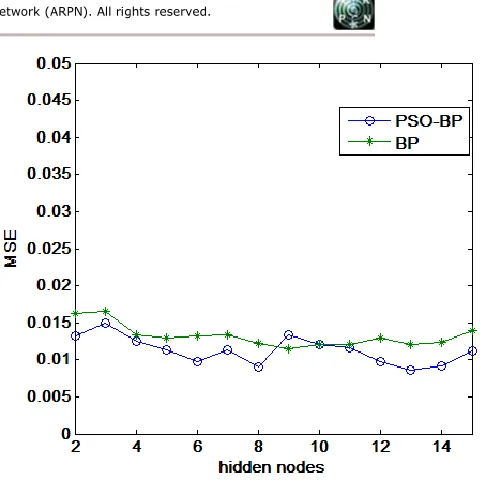
Figure 4 shows the relation of the number of hidden nodes and the testing MSE for both PSO-BP and BP algorithm. As an overall results, the MSE for the PSO-BP algorithm is lesser than the BP algorithm.

PSO-BP algorithm manage to acquire a better percentage accuracy than the BP algorithm as seen in Figure 5. PSO-BP algorithm achieved the highest accuracy of 88% with hidden nodes of 3 while the BP algorithm only achieved 81.3% with 4 hidden nodes, as shown as in Table 1.

Figure 4: MSE for PSO-BP and BP algorithm.

Figure 5: Percentage of accuracy for PSO-BP and BP algorithm.

CONCLUSION

PSO algorithm has a good global searching ability, but has a tendency to stuck onto the global minima while the BP algorithm has a good local searching ability, but often stuck in the local minima. By combining both algorithm, the PSO-BP algorithm has proven its effectiveness by showing a worthy improvement for the system to classify the non-linearly separable data of the surface texture images from the standard BP algorithm. It manages to reduce the probability of getting stuck on the global and local minima.

ACKNOWLEDGEMENT

Management (ORICC), University Tun Hussein Onn Malaysia is gratefully acknowledged.

REFERENCE

Han, F., Gu, T. and Ju, S., 2011. An Improved Hybrid Algorithm Based on PSO and BP for Feedforward Neural Networks. , 5(2), pp.106–115.

Hao, S., 2009. An “ Mushroom Recognition System ” based on Matlab and QuickCog.

Haralick, R.M., Shanmugam, and K., Dinstein, I., 1973. Textural Features for Image Classification. IEEE Transactions on Systems, Man, and Cybernetics, 3(6), pp. 610–621.

Khan, K. and Sahai, A., 2012. A Comparison of BA, GA, PSO, BP and LM for Training Feed forward Neural Networks in e-Learning Context. International Journal of Intelligent Systems and Applications, 4(7), pp.23–29.

Liu, J. and Qiu, X., 2009. A Novel Hybrid PSO-BP Algorithm for Neural Network Training. 2009 International Joint Conference on Computational Sciences and Optimization, (1), pp.300–303.

Mahamad, A.K., Saon, S., Ramli, H., Zainudin, F.L., and Yahya, M.N., 2014. Identification of Material Surface Features using Gray Level Co-Occurrence Matrix and Generalized Regression Neural Network. , 8th MUCET 2014,

Date: 10-11 November 2014, Melaka, Malaysia, pp.10–11.

Ren, J. and Yang, S., 2010. An Improved PSO-BP Network Model. 2010 Third International Symposium on Information Science and Engineering, 2(4), pp.426–429.

Suhaila, S., Hazli, R., Shimamura, T., 2013. Smooth region's mean deviation-based denoising method, International Journal of Circuits, Systems and Signal Processing, 7(3), pp.191-198.

Singh, N. and Singh, S.B., 2012. Personal Best Position Particle Swarm Optimization, 12(6), pp.69–76.

Tahmasbi, A., Saki, F. and Shokouhi, S.B., 2011. Classification of benign and malignant masses based on Zernike moments. Computers in biology and medicine, 41(8), pp.726–35.

Zainudin, F.L., Mahamad, A.K., Saon, S., and Yahya, M.N., 2014. Comparison between GLCM and Modified Zernike Moments for Material Surfaces Identification from Photo Images. , 2014, pp.1–4.