Mining GPS logs to augment location models

Mining GPS logs to augment location 

models

Saraee, MH and Yamaner, S

Title

Mining GPS logs to augment location models

Authors

Saraee, MH and Yamaner, S

Type

Conference or Workshop Item

URL

This version is available at: http://usir.salford.ac.uk/18849/

Published Date

2005

USIR is a digital collection of the research output of the University of Salford. Where copyright 

permits, full text material held in the repository is made freely available online and can be read, 

downloaded and copied for non­commercial private study or research purposes. Please check the 

manuscript for any further copyright restrictions.

Mining GPS logs to augment location models

M. Saraee & S. Yamaner

University of Salford, UK

Abstract

The availability of mobile computing and satellite technologies make it possible to develop applications that are aware of user location. However, as the amount of collected data grows quickly, coming up with techniques that ease interpretation of such data is essential. In this paper, we employ a data mining approach to infer regularly visited locations and the routes between them from GPS (Global Positioning System) logs captured in an incremental fashion by a PDA. In our implementation, outdoor locations can be detected as well indoor locations visited by the users. Once the list of locations is determined, this list is clustered to group locations in close proximity. After clustering and reduction, the original database is scanned for transitions between location groups to find the routes. If there are similar routes between origin and destination then these will be merged, and finally a list of different routes between two locations will be obtained. This technique could be used as part of a monitoring system for vehicles that are aware of their location and security as well as using logs from different users to create a dynamic map of the regions where digital maps are not available or not feasible.

Keywords: PDA, GPS, data mining, time series, clustering, route determination.

1 Introduction

Due to the public availability of GPS systems and also powerful mobile computing devices, location based computing has become one of the most attractive research topics in Computer Science and Telecommunications. There have been several context-aware tourism information systems such as Cyberguide (Abowd et al. [1]) from Georgia Institute of Technology, and GUIDE (Cheverst et al. [2]) project from Lancaster University. In addition, many commercial products exist that aim at providing journey planning and routing information to mobile phones and Personal Digital Assistants (PDAs). The easier it gets to collect location data, the harder it gets to make sense of it. In addition to massive amounts of information, the GPS system also introduces some errors, and it is essential to develop techniques that can handle such information in ways that return the most meaningful results possible.

The aim of this paper is to introduce the approach taken to collect GPS data from mobile units, then process the logs to determine locations relevant to the user of the system, and visualise the routes taken between those locations. The following section provides background to relevant research. After the background section, discussion of the design of the system is presented, followed by an outline of implementation issues. In the conclusion section, the current state of the system is discussed and future works are outlined.

2 Background

Global Positioning System (GPS) is the name of a system that is able to show the position of special receivers on Earth at any time, anywhere. GPS satellites orbit 11,000 nautical miles above Earth (French [3]). They are monitored continuously at ground stations located around the world. The satellites transmit signals that can be detected by anyone with a GPS receiver. GPS receivers detect, decode and process GPS satellite signals. The principle behind GPS is the measurement of distance (or “range”) between the satellites and the receiver. The satellites tell exactly where they are in their orbits. When the GPS unit receives signals from at least three satellites, the location of the GPS unit can be visualised as the intersection point of three circles that have radius equal to distance between the unit and each of the satellites. The GPS receiver processes the satellite range measurements and produces its position. Simply, the GPS system consists of satellites whose paths are monitored by ground stations. Each satellite generates radio signals that allow a receiver to estimate the satellite location and distance between the satellite and the receiver. The receiver uses the measurements to calculate where on or above Earth the user is located.

Wolf et al. [5] have used GPS loggers in hundreds of cars in three Swedish Cities and observed these vehicles for up to two years. For this study, speed and location data have been uploaded to servers at regular intervals for later analysis. By analysing the data, they have extracted trip purposes as well as traveller behaviour patterns of those included in the study.

In a different research effort, Marmasse and Schmandt [6] have developed a computing environment that links personal information to locations in people’s lives. The system learns about the location a user visits frequently by monitoring signal loss for a period of time, and once locations are determined, makes it possible for the user to associate “to do” notes with those locations. In addition, they have also provided a route-learning component that can infer the routes between popular places.

Patterson et al. [7] also used GPS logs to infer transportation models of users. Their technique can learn the transportation model of the user as well as the most likely route in an unsupervised manner.

3 System

overview

The system described in this paper consists of a server component exposed as a web service, and a client component that runs on an iPAQ PDA with GPS support. The equipment involved in the system design is as follows:

• HP iPAQ 5450 PDA with wireless network and Bluetooth support

• Fortuna Xtrack Compact Flash and Bluetooth GPS units

• A desktop server connected to the Internet acting as a server Software environment used:

• Windows XP Professional on desktop and Pocket PC 2003 on PDA

• Microsoft SQL server on desktop and SQL server CE on PDA

• Microsoft Visual Studio 2003 as development environment and C# as programming language

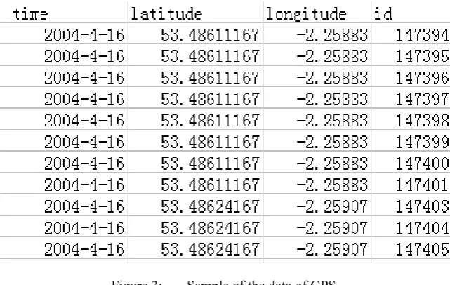
The client application uses a SQL Server CE database to store user’s GPS log. When an Internet connection is available, the user can send the GPS log to the server and restart capturing data. The data is collected in an incremental fashion and can be sent to the server at any time the user feels convenient.

Initially the data collection strategy was similar to Ashbrook and Starner’s [4, 8] work; if the user is moving faster than a speed threshold (>1.5 Km/h) the system would start logging GPS output until user stops or reception is lost. In the later stages of development we adopted a different approach, and GPS output was logged regardless of the speed. The reason behind this change is explained in detail in the implementation section.

In addition to determining locations, the system can also determine the unique routes taken between any two locations in the user’s location model. We have defined a route as a transition between two known locations that start and end within a time frame. The routes are handled as one way, therefore route AÆB is not treated as route BÆA even though they might be the same.

4 System

implementation

4.1 Clustering algorithm

In order to represent locations appropriately, clustering the data into location groups plays an important role. In our application, we have used clustering for two main reasons. The first functionality of clustering used is for grouping the locations in close proximity together that are within a time window. Therefore clustering is the central part of determining outdoor locations. Details of this approach are discussed in the following section. Secondly, clustering is used after determining indoor and outdoor locations. This time clustering is used to group locations that are close to each other together. This way our location list can be revised and only unique locations will be included in the final list. This is essential because in many cases the GPS system will introduce errors and report the same location as different coordinates. In addition, the “locations” as we call them are not simply precise points but rather buildings or fields that are somewhat relevant to our lives.

In order to represent locations consistently, a variation of the distance based clustering algorithm K-Means has been implemented in a similar way to Ashbrook and Starner’s [4, 8] implementation. We take the first location that is not clustered in the data set and then take every point that is within a fixed distance from that point. Once they are grouped, the mean of this group is taken in terms of latitude and longitude. Then all points that are within the specified distance are selected, and the mean is calculated one more time. This loop continues until the mean stops moving. Once the mean stops changing, we add this mean to our clusters list and then select the next point from the original set of points that is not yet a member of a cluster.

4.2 Determining places

In order to determine the locations that are relevant to users from the GPS log, we have implemented two different approaches. We have followed a similar approach to Ashbrook and Starner’s [4, 8] work to determine indoor locations. In addition, we have also implemented a moving time window based algorithm for determining outdoor locations where GPS signal is not lost and captured continuously.

leaves, there will be a time gap between the point where signal is lost and the point where the signal is regained after leaving the building. This idea forms the basis of the algorithm used in various research projects [4, 6, 8].

In order to implement this principle, we have analysed the entries in the database and looked for time gaps between two consecutive readings. If there is a time gap greater than a predefined time threshold, then it means either the user has entered a building and then stayed there for a particular period of time, or the GPS signal was lost. Looking at the frequency of determined places, locations that occur less frequently are eliminated from the locations list as it might hint GPS signal losses. Considering that it is quite unlikely to have GPS signal problems in the same place many times, this seems to be a safe assumption. As a result, if there are frequently visited locations where the time gap is greater than a predefined threshold, those spots are considered as candidate locations and remain in the list.

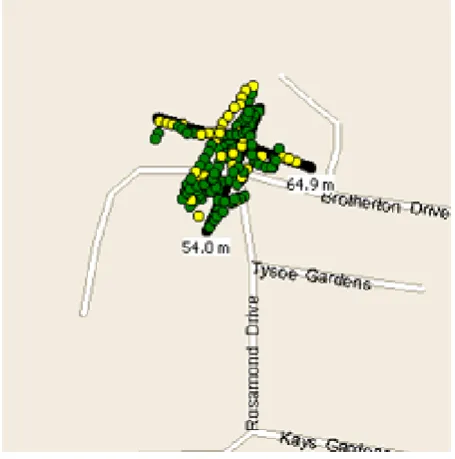
Coupled with the data collection strategy outlined earlier, this approach is ideal for determining indoor locations (looking for signal loss). On the other hand, it is not quite appropriate for determining outdoor locations. Even though data to be logged is filtered by minimum speed, the nature of GPS makes this approach less practical. It should be expected that a stationary GPS unit will in many cases report the device is moving, and therefore data logging will continue, and in the end such locations will not be visible to the algorithm outlined above. As shown below in Figure 1, even though the GPS unit is stationary, the output shows the device moving up to thirty meters away from the real position.

Therefore, after analysing the data with the initial algorithm, we have implemented a different algorithm that is based upon a moving time windows concept. As long as there is satellite reception, even if the user stands still, the GPS unit will report motion from time to time. Taking a constant time window, analysing and clustering all the readings within the window as described before, we can expect so see more than one cluster even if the user did not move for the duration of time window. Even though there may be errors in GPS output, in many cases GPS readings will concentrate around the real position. Therefore, if the user remained in the same location we should see at least one or more clusters in the current window and the cluster with most elements should include the majority of the points in the window.

We implement this idea by taking a time window of fifteen minutes and then move through the database and calculate clusters for every time window. The distance used to calculate the clusters is fifty meters. Even though most of the time GPS errors will be less than fifteen meters, fifty meters distance is more realistic and likely to tolerate GPS errors to avoid having many clusters that partly include same location.

All clusters are looped through to find the cluster that has maximum number of elements. Once this cluster is selected, then the number of elements in this cluster is divided by total number of elements in the window. If the result is greater than 60%, and the total number of elements in the window is greater than a predetermined threshold, we finally check the time span between the first and last element in the window to make sure there are enough readings in the current window. If the time span is greater than ten minutes (time threshold), we conclude that this is a location and move the window. We repeat this process, ignoring the location if it is close to a previously determined location, then move the window again. This loop continues until the end of the database is reached. Finally, at the end of this procedure, locations that would not be visible in a time gap based algorithm will be determined. Now that we have two different sets of locations, we need to merge these two sets to have the final locations list. The readings have timestamp information and therefore two sets of data can be merged by looping through each set. Once data is merged, we then use the clustering algorithm again to find the location clusters.

Time Threshold and Number of Locations

00:00:00 00:07:12 00:14:24 00:21:36 00:28:48 00:36:00 00:43:12 00:50:24 00:57:36 01:04:48 01:12:00 01:19:12 01:26:24 01:33:36 01:40:48 01:48:00 01:55:12

15 30 35 41 45 51 59 67 68 88 ₁₄2 ₁₈6 ₃₁3 2126

Number of Locations

Ti

m

e

T

re

shol

d (

h

h:

m

m

:s

s

)

Figure 2: Relationship between number of locations and time threshold.

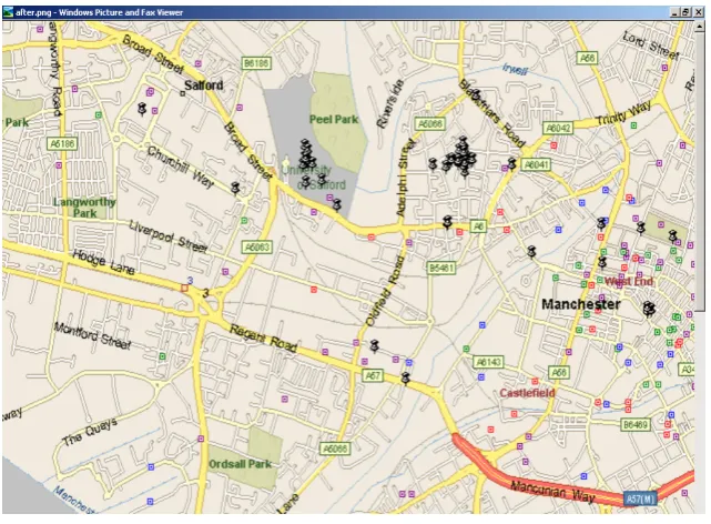
Figure 4: The map of user’s route before data mining.

4.3 Determining routes

Once the locations that are relevant to the user have been determined, the database is then scanned for transitions between these locations. For simplicity, we currently define a route as a number of sequentially ordered GPS coordinates (nodes) that are between two known locations and the time span between from starting and ending is within the predefined journey time threshold.

To find out the routes, the database is scanned to find the first occurrence of an origin. Once this is found, we then select the last reading that belongs to the same cluster with this origin and then start looping though the database to find the first instance of a destination. Once a destination is found, the time gap between two readings is calculated, and if time gap is less than for example an hour then we select these points and add them to the AÆB route list. Then in the same database, we look for the second occurrence of an origin and the first occurrence of a destination and so on. If we find more routes between same destination and origin, we then compare the route with the routes in the list. If the routes are similar then they are merged together, and if they are different a new route will be added to the AÆB routes list.

Similarity between the routes is measured by comparing the nodes between two candidate routes. If the majority of nodes have at least one node in the other route candidate, then we conclude these are similar and merge them. If the nodes are different then these routes are perceived as distinct routes.

After defining the routes, the last step is reducing the number of nodes that form a route. The reduction process is straightforward. We simply reduce the nodes based on their distance to previous nodes. In our experiments, we have used 50 meters as distance between nodes, however we are planning to use heading information logged from GPS unit for more realistic reduction. Instead of using the distance as the only determinant, we will be using the variation in heading information. The nodes will be ignored until there is significant change in heading, and this algorithm should provide more accurate routes which also require less data storage.

5 Conclusion and future work

After analysing GPS data and clustering them with a predefined time threshold and time windows, we are able to determine the locations in which the GPS user has spend most of their time. We have successfully improved location the discovery algorithm so that it is possible to discover locations where the GPS device keeps on logging information. This makes it possible to catch locations that would be invisible otherwise.

In addition to finding the relevant locations to users, we can also define how they travel between these locations and therefore it is possible to predict the destination by considering previous location and current route. Discovering the routes preferred by users provide opportunities such as information delivery about the routes, before the user is stranded in traffic or various condition that might arise in city life. This information is also useful to understand traffic patterns of individuals and develop or improve services to make city life easier. The news about UK government’s future plans to introduce road taxes based on usage patterns, and an insurance company’s tests regarding introducing different rates based on the routes their customers use, are only two examples to prove how important it is to collect and analyse location data to develop future services.

We have therefore introduced our simplified approach to achieve the objectives outlined, and in the future we are planning to improve route detection functionality to be able to detect sub routes. In addition, the route reduction algorithm will also be improved to achieve better representation of the routes.

References

[1] Abowd, G.D., Atkeson, C.G. et al, Cyberguide: A mobile context-aware tour guide. Wireless Networks, 3(5), pp. 421–433, 1997.

[2] Cheverst, K., Davies, N. et al, Developing a context-aware electronic tourist guide: some issues and experiences. Conference on Human Factors and Computing Systems, The Hague, The Netherlands, ACM Press New York, NY, USA, 2000.

[3] French, G.T., Understanding the GPS; an Introduction to the Global Positioning System; What It Is and How It Works, Bethesda, MD, GeoReseach Inc, 1996.

[4] Ashbrook, D. and Starner, T., Learning Significant Locations and Predicting User Movement with GPS. IEEE Computer Society, 2002. [5] Wolf, J., Schoenfelder, S. et al, Eighty Weeks of Global Positioning

System Traces: Approaches to Enriching Trip Information. Emerging Travel Data Collection and Monitoring Techniques, Washington, D.C., Transportation Research Board, 2004.

[6] Marmasse, N. and Schmandt, C., Location-aware information delivery with commotion, Cambridge, MA, MIT Media Laboratory, 2000.

[7] Patterson, D.J., Liao, L. et al, Inferring High-Level Behavior from Low-Level Sensors. Fifth Annual Conference on Ubiquitous Computing, Seattle, WA, Springer-Verlag Heidelberg, 2003.

[8] Ashbrook, D. and Starner, T., Using GPS to learn significant locations and predict movement across multiple users. Personal and Ubiquitous Computing, 7(5), pp. 275–286, 2003.

[9] Choi, E. and Cicci, D.A., Analysis of GPS static positioning problems.