First-order estimates of the costs, input-output energy analysis, and energy returns on investment of conventional and emerging biofuels feedstocks

(1)

* Corresponding author at: Tel.: +1 515 451 0859 E-mail address: [email protected]

Please cite this article as: Christiansen K., Raman D.R., Hu G., Anex R. First-order estimates of the costs, input-output energy analysis, and energy returns on investment of conventional and emerging biorenewable feedstocks. Biofuel Research Journal 20 (2018) 894-899. DOI: 10.18331/BRJ2018.5.4.4

Biofuel Research Journal 20 (2018) 894-899

Original Research Paper

First-order estimates of the costs, input-output energy analysis, and energy returns on

investment of conventional and emerging biofuels feedstocks

Katrina Christiansen

1,

_{*, David Raj Raman}

2

_{, Guiping Hu}

3

_{, Robert Anex}

4

1_{Stalende, LLC 310 4}th_{Ave SE Jamestown, ND 58401, USA.}

2_{Department of Agricultural and Biosystems Engineering, Iowa State University, Ames, IA 50011, USA.}

3_{Department of Industrial and Manufacturing Systems Engineering, Iowa State University, Ames, IA, 50011, USA.} 4_{Department of Biological Systems Engineering, University of Wisconsin, Madison, WI, USA.}

HIGHLIGHTS

Compared fuel production metrics from various biomass feedstocks.

Estimated the carbon equivalent emissions associated with biofuel produciton.

Predicted algae biomass production rates of 120 MG/(ha.a), ten times greater than Maize.

Predicted algae biofuel costs ranging from 28 to 65 US $/GJ compared to 17 US $/GJ for Maize ethanol.

Estimated biofuel energy returns on investment near zero for algae and 25 for Switchgrass.

GRAPHICAL ABSTRACT

           

ARTICLE INFO ABSTRACT

Article history:

Received31July2018

Received in revised form 28September2018 Accepted8October2018

Available online1 December2018

Keywords:

Algae Biofuel Biomass feedstocks Bioenergy LCA

Input-output analysis

Here we report on a static, algebraic, spreadsheet-implemented modeling approach to estimate the costs, energy inputs and outputs, and global warming potential of biomass feedstocks. Inputs to the model included literature sourced data for: environmental factors, crop physiological-parameters such as radiation use efficiency and water use efficiency, and crop cost components. Using an energy-input-output life-cycle-assessment approach, we calculated the energy associated with each cost component, allowing an estimate of the total energy required to produce the crop and fuel alongside the energy return on investment. We did this for crop scenarios in the upper Midwest US and Far West US (for algae). Our results suggested that algae are capable of the highest areal biomass production rates of 120 MG/(ha·a), ten times greater than Maize. Algal fuel systems had the highest costs, ranging from 28 to 65US $/GJ, compared to 17 US $/GJ for Maize ethanol. Algal fuel systems had the lowest energy returns on investment, nearly 0, compared to 25 for Switchgrass to ethanol. The carbon equivalent emissions associated with the production schemes predictions ranged from 40 (Maize) to 180 (algae PBR) CO2eq/GJnet. The

promise of low cost fuel and carbon neutrality from algae is demonstrated here to be extremely challenging for fundamental reasons related to the capital-intensive nature of the cultivation system.

(2)

Christiansen et al. / Biofuel Research Journal 20 (2018) 894-899

1. Introduction

Photosynthetically-derived carbon will provide critical material and energy resources for humanity in the 21st_{century, and beyond. Furthermore, barring} catastrophes, the demand for these resources will rise as human populations increase, standards of living increase, and non-renewable (i.e., fossil) carbon sources are depleted. The environmentally-sustainable and cost-effective production of biorenewable carbon is therefore one of several defining challenges for our species in this century. Tackling this challenge will involve an array of approaches including developing novel plants and cropping systems and optimizing landscape design to meet human needs, and will be facilitated by robust estimates of the cost, energy requirements, and environmental impacts of various biomass resources are critical.

The scientific consensus that anthropogenic global warming is occurring (Carlton et al., 2015; Cook et al., 2016) has driven a multitude of approaches to reducing the carbon-intensity of modern industrial society (Leung et al., 2014; Huisingh et al., 2016). Although the likelihood is low that these approaches, even collectively, can stave off major climate changes that will severely impact existing global agricultural production (Schuur et al., 2008; Gornall et al., 2010; Jaggard et al., 2010; Lesk et al., 2016), such approaches are still worthy of exploration as they can be part of an effort to reduce the degree of warming that ultimately occurs (Pacala, et al., 2004). One existing yet controversial approach (Keyzer et al., 2008; Tomei and Helliwell, 2016) to reducing anthropogenic greenhouse gas emissions is by replacing fossil-based liquid transportation fuels (primarily gasoline and diesel) with similar or identical fuels derived from biomass resources (Wang, 1999; Richard, 2010). Brazil makes 22% of its transportation energy from sugarcane-derived ethanol – totaling approximately 31 × 109_{L annually (}_{FAO, 2015}_{) – while the US}

makes over 13% of its gasoline volume from Maize-starch-derived ethanol – totaling approximately 56 ×109_{L annually (}_{EIA, 2016}_{). The economic} and environmental viability of these biofuels have been questioned for at least the last two decades (Hill et al., 2006; Gomiero et al., 2015), with concerns on issues such as competition between human food and vehicle fuel needs, water quality impacts of increasingly intensive management practices, and air quality and wildlife habitat impacts from changing land-use patterns (Hill et al., 2016; Otto et al., 2016). In addition to a strong debate on these claims in the scientific literature, some have sought to address the weaknesses of starch-ethanol by developing biofuel production systems that convert into fuel the lignocellulosic portion of Maize, or the lignocellulosic biomass derived from perennial crops, or the oil and lignocellulosic biomass formed by microalgae (Pienkos and Darzins, 2009). This plethora of approaches to biofuel production has made it difficult to understand the fundamental performance of and barriers to these different feedstocks. The purpose of this study was to use a generalized modeling approach to provide insight into the strengths and weaknesses of these potential technologies.

2. Materials and Methods

The model implements an algebraic, static, approach to estimating productivity and cost of biomass feedstocks detailed in the model available here (https://works.bepress.com/raj_raman/64/). The overall computational approach for any feedstock is the same and is as follows: Compute a solar-energy-limited maximum carbon-capture based upon growing-season solar energy inputs and literature reported radiation use efficiency (RUE). In parallel, compute a water-limited maximum carbon-capture based upon growing-season rainfall and literature reported maximum water use efficiency (WUE). De-rate both maximum carbon-capture estimates to account for critical losses including respiration and non-harvestable fraction, to estimate a maximum light-limited and water-limited yield; select the lower of the two to estimate the maximum biomass yield. Use the maximum biomass yield to calculate theoretical energy yield based on biomass energy content, as well as maximum biofuel yields based upon literature estimates of conversion efficiencies from biomass to fuel. The

Supplementary Methodology “Framework for the Evaluation of Biomass Energy Feedstocks (FEBEF)” describes the calculations in detail.

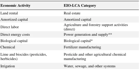
To estimate costs, the FEBEF divides the cost of production and fuel conversion into nine primary line-items that are inclusive of both terrestrial and aquatic feedstocks, namely: land rental, amortized capital, direct labor, direct energy, biological capital, macronutrients, lime and biocides, irrigation, and carbon dioxide. These costs are expressed on a per unit land area basis, as literature estimates inform their values. All costs except algae capital costs scale by yield to reflect that higher yield typically requires more inputs and occurs on higher value land (e.g., Clark et al., 1999; Lobell et al., 2009). Algae capital costs scale by area rather than yield.

The model uses an economic-input-output-life-cycle-analysis approach to compute the embedded energy and greenhouse-gas emissions from each cost line-item (Carnegie Mellon University Green Design Institute, 2008) in 2015 dollars customized for Iowa. The sum of these allows a first-order estimate of the total embedded energy as well as of the greenhouse gas (GHG) emission associated with feedstock production.

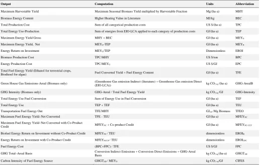
With maximum yield, biomass cost, energy input, and GHG emissions available for each feedstock, FEBEF computes key performance indicators such as: Gross Maximum Energy Yield (GJ/(ha·a)), Energy Return on Investment (EROI, dimensionless), and Biomass Production Cost (US $/ton, US $/Mg). Furthermore, based upon the biomass-to-fuel conversion parameters, FEBEF computes other additional key performance indicators including Net Maximum Fuel Energy Yield (GJ/(ha·a)), Fuel Energy Cost (US $/GJ), and Carbon Intensity of Fuel Energy Source (kg CO2 eq/GJ). A summary of the computations and categories is given Table 1.

3. Results and Discussion

3.1. Model biomass outputs

The model Maximum Harvested Yields (MHY) as predicted by radiation or water use limited computation are shown in Figure 1

and compared

to

Abbreviations

AZ Arizona

bbl Barrel

BRY Best Reported Yield

CC Cost of Conversion

CCFEP Cost for Conversion of Fuel Energy Produced

CFEP Cost for Fuel Energy Produced

CIES Carbon Intensity of Energy Source

CIFES Carbon Intensity of Fuel Energy Source

CO2 eq Carbon Dioxide Equivalent

EC Energy Cost

ECB Energy Content Of Biodiesel

EIO-LCA Economic Input-Output Life Cycle Assessment

EROI Energy Return on Investment

FEBEF Framework for the Evaluation of Biomass Energy Feedstocks

HI Haiwaii

GHG Greenhouse Gas

MFEYNC Maximum Fuel Energy Yield-Net Converted

MG Megagram

MHY Maximum Harvestable Yield

NM New Mexico

ORP Open Raceway Pond

PAR Photosynthetically Available Radiation

PBR Photobioreactors

PV Photovoltaic

RMHY Ratio of Max Light to Max Water Yields

RUE Radiation Use Efficiency

TCFEP Total Cost for Fuel Energy Produced

TCP Total Cost for Production

TEC Total Energy Cost

TEU Total Energy Use

TEUC Total Energy Use for Conversion

TEUP Total Energy Use for Production

TEUPC Total Energy Use for Production and Conversion

TFEO Transportation Fuel Energy Out

TFEY Total Fuel Energy Yield

WUE Water Use Efficiency

(3)

Fig. 1. The model estimates of maximum harvestable yield (MHY, Mg/(ha.a)) for each of the seven systems is shown as dark bars alongside the best reported yields (BRY, Mg/(ha.a)) for the same case (light bars). Approximate collection areas and durations of the BRY values are provided for context (*: Extrapolated from 2-Yeat Seasonal Average; **: Extrapolated from daily maximum; ***: Extrapolated from historic maximum).

Best Reported Yields (BRY) from literature. In many cases, the model appears conservative with slightly higher yields reported than predicted.

In contrast, when considering large-area averages, actual yields are predictably lower, for example, the 2015 Maize grain yield was 12 Mg/ha in Iowa and 10.5 Mg/ha in the US overall, or roughly half the maximum predicted. But the US overall yield reflects performance over some 32.6 ×106_{ha of cropland. The claims by algal fuel proponents regarding the} superior yield potential is supported by the best-reported yields and the model predicted MHY. Continuous yield data sets from commercial or large research scale production are scarce for algae as well as for Switchgrass and Miscanthus, they were therefore extrapolated from short-term and/or small-scale results for comparison. As reflected in the divergence between large-scale and small plot Maize yields, caution should be used in presuming that such yields could actually be realized at present in full-scale systems. Algal production systems have the advantage of continuous harvest and production, as well as of not leaving inaccessible (non-harvestable) biomass underground. This drives their impressive areal biomass annual yields, which are more than double the terrestrial crops. Furthermore, our results suggest that algae are RUE limited, in contrast to the non-irrigated terrestrial crops we modeled which are WUE limited. Maize, however, has lower respiration carbon losses (20%) (Taylor, 1998) than algae, (25%) (Christi, 2007). All the terrestrial crops invest carbon in unharvested root biomass, lose carbon to soil through root exudates, and also have an unharvested biomass above ground. All these biological, agricultural, and mechanical differences lead to huge calculated differences in the total fixed carbohydrate by the plants; Algae fixing 71%, Maize (Grain) 35%, Maize (Grain +Stover) 53%, Switchgrass 34%, and

Output Computation Units Abbreviation

Maximum Harvestable Yield Maximum Seasonal Biomass Yield multiplied by Harvestable Fraction Mg/(ha·a) MHY

Biomass Energy Content Higher Heating Value in Literature MJ/kg BEC

Total Production Cost Sum of all categorical production costs US $/(ha·a) TPC

Total Energy Use-Production Sum of energies from EIO-LCA applied to each category of production costs GJ/(ha·a) TEP

Maximum Energy Yield Gross MHY × BEC GJ/(ha·a) MEYG

Maximum Energy Yield, Net MEYG-TEP GJ/(ha·a) MEYN

Energy Return on Investment MEYG/TEP Dimensionless EROI

Biomass Production Cost TPC/MHY US $/ton BPC

Energy Production Cost TPC/MEYG US $/GJ EPC

Total Fuel Energy Yield (Ethanol for terrestrial crops,

Biodiesel for algae) Fuel Converted Yield × Fuel Energy Content GJ/(ha·a) TFE

Green House Gas Emissions-Areal (Biomass only) (Greenhouse Gas emission Indirect (literature) + Greenhouse Gas emission Direct

(EIO-LCA)) kg CO2 eq /(ha·a) GHG-ArealB

GHG Intensity (Biomass only) GHG-Areal / Total Fuel Energy Yield kg CO2 eq /GJ GHG-Intensity

Total Energy Use Fuel Conversion Sum of Energy Use in Fuel Conversion GJ/(ha·a) TEF

Total Energy Use TEP + TEF GJ/(ha·a) TEU

Transportation Fuel Energy Out TFE/MHY GJout /Mg Biomass TFEO

Maximum Fuel Energy Yield–Net Converted TFE - TEU GJ/(ha·a) MFEYNC

Maximum Fuel Energy Yield–Net Converted with Co-Product

Credit MFEYNC + Co-product Credit GJ/(ha·a) MFEYNC-CCP

Biofuel Energy Return on Investment without Co-Product Credit MFEYNC / TEU dimensionless EROIB

Energy Return on Investment with Co-Product Credit MFEYNCCP / TEU dimensionless EROICPC

Fuel Energy Cost (BPC+FPC) / TFE US $/GJ FPC

GHG Total–Areal Basis Conversion Indirect Emissions + Conversion Direct Emissions + GHG-Areal _Basis kg CO2 eq/(ha·a) GHGTAB

Carbon Intensity of Fuel Energy Source GHGTAB / MEYN kg CO2eq/GJ CIFES

896

Table 1.

(4)

Miscanthus 27%. These processes and practices lead to the biomass yield advantage carried by algae.

Interestingly, Maize grain plus stover outperforms the other cellulosic crops. For terrestrial crop yields to approach the BRYs on a broad scale, growers would have to replicate the intensive farming practices done at the small scale while the algal production would have to overcome the challenges of exponential growth and lag phase cycles to maintain high yield consistently on an annual basis.

3.2. Annual energy production (raw biomass)

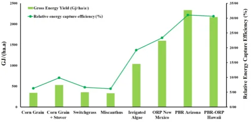
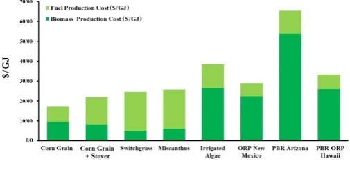
Combining the yield data with assumptions regarding biomass energy density results is an estimate of the annual gross energy production for each system. To contextualize these values, the values are also expressed on the basis of percentage of total annual site solar radiation collected as shown in Figure 2. The gross energy yield tracks closely to the relative energy capture (ratio of energy capture GJ/(ha·a) to solar radiation GJ/(ha·a)) for all production scenarios. The benefit of an extended production season with the three southern algal production scenarios as well as being photosynthetically limited in carbon capture lead to the marked differential in energy yield with the terrestrial crops. In contrast are the biomass production costs, it is far more expensive to make biomass in aquatic schemes than terrestrial as shown in Figure 3. Aquatic systems have large capital costs as well as high labor costs and direct energy costs for centrifugation and cooling. The photobioreactor (PBR) system much more so, resulting in biomass production costs tens time more than the terrestrial and double the other algal scenarios.

Fig. 2. Gross Energy Production Yield (GJ/(ha.a)) and Relative Energy Capture Efficiency (%).

Thesealgae biomass production values are lower than the minimum selling price reported in the Billion Ton report (719-2998 US $/dry ton) (US DOE, 2016).The lowest cost production crop, Switchgrass, is due mostly to the lower land rental costs associated with marginal land in addition to being a perennial. The biomass production costs between the perennial crops are 30% to 45% lower than the annual Maize crop. While there is an established stand cost advantage for perennial crops, there is also the risk the growers assumeby delaying planting of a genetically improved cropevery year as one can do with Maize.

Fig. 3. Biomass production costs for the terrestrial and algal production scenarios.

It is important for bioenergy proponents to be cognizant of the constantly increasing efficiency of photovoltaic (PV) cells. These systems have seen a 0.3% annual increase in efficiency (Detwiler, 2013) with disruptive technologies leading to huge increase of 7% efficiency (Mearian, 2015) over current commercial cells, much greater than the 1% annual rate of yield increase of Maize (Neilsen, 2012). Furthermore, commercially available PV are now achieving efficiencies ca. 25%, which is greater than all but the algal systems we modeled. Moreover, while all practical energy systems are subject to various storage, transport, and conversion losses, from a vehicle-propulsion standpoint, PV-based electric vehicles have a significant advantage, as shown in Table 2.

As tabulated in Table 2, current PV systems can achieve photon-to-wheel efficiencies on the order of 20%. This is over seven times greater than the best widely commercially available scenario for biofuel. At present, no rechargeable battery comes within an order of magnitude of the energy density achieved by ethanol or biodiesel. The benefits of such high energy densities are diminishing for surface vehicles, as increasing efficiency leads to reduced total energy storage needs, and improved materials lead to ever lighter structures which “make room” for heavier energy storage systems. But in long-haul aviation, the benefits of high energy density are harder to overcome, thus justifying the strategy of aviation-biofuels.

While the fuel conversion costs of oil to biodiesel are less than for lignocellulosic biomass to ethanol, the total energy cost for algal biofuels systems is still greater than that for terrestrial crops biofuels, as shown in Figure 4. Algal fuel technologies suffer from both high capital and operating costs. The impact of marginal land costs, lower crop inputs and water use efficiencies drive the low cost energy option to be Switchgrass. However, the cost of conversion for the lignocellulosic crops pushes the total energy cost for Switchgrass above that of Maize. This is not surprising and tracks the experience of the US ethanol industry in which slightly over 200 starch/sugar ethanol plants currently produce 15.7 billion gallons of ethanol annually, while 15 cellulosic plants produce a total of 0.1 B gallons annually (Ethanol Producer Magazine, 2018). This 150-fold volume

Table 2.

Photon to wheel efficiencies for selected crops, as well as for photovoltaic-supplied battery electric vehicles. (Source: http://www.cleancaroptions.com/html/energy_efficiency.html)

System Photon-Fuel Efficiency(%) Fuel-Wheel Efficiency(%) Overall Efficiency (Photon-Wheel)(%) Fuel Energy Density (MJ/kg)

Maize Grain to Gas ICE 7 23 1.6 26.4

Maize Grain to Hybr. ICE 7 40 2.8 26.4

Maize Grain + Stover to Gas ICE 10 23 2.3 26.4

Maize Grain + Stover to Hybr. ICE 10 40 4.0 26.4

Best-Case Algae to Gas ICE 30 23 6.9 42.2

Best-Case Algae to Hybr. ICE 30 40 12.0 42.2

Photovoltaic to BEV 25 85 21.3 ~1.0

(5)

Fig. 4. Total Energy Production Costs ($/GJ) summed from biomass production cost and fuel production cost. Dark horizontal vertical line at left to range of gasoline prices (pre-tax) from 2012 –2018 projected (Source: EIA 2018; https://www.eia.gov/outlooks/steo/report/us_oil.cfm).

difference is significant and serves as an industrial indicator of biological challenges of degrading cellulose and lignin into fermentable sugars. While there have been technological advancements made in the conversion of cellulose to ethanol (Singh et al., 2015_{), there has yet to be a disruptive}

technology that halves the cost of conversion in tandem with reducing the cost of transporting lower energy dense, cellulosic feedstock to plants at larger radii (Hess, 2007). The cost of fuel from algae is not cost competitive with the ethanol feedstocks due to the high capital and labor costs even though the cost of biodiesel conversion is less than Maize ethanol. Predicted algal fuel costs are 30% more than the terrestrial crop fuels even though there is 1.5 times more energy density in biodiesel than ethanol. The low cost of ethanol from Switchgrass is due to the low production costs. It is difficult for ethanol and biodiesel to compete in the fuel market until oil exceeds a variable breakeven point (US $/bbl) given the dependencies of crude oil, gasoline, ethanol, corn, and Distiller Grains prices alongside oxygenate premiums and government subsidies.

When we examine the energy production cost for algal systems as function of interest rate on the capital, we see that there is a meaningful increase from 0% interest to 5% and then 10%. The internal rate of return and discount rate of 10% is adopted from Efroymson et al. (2016). This is higher than the discount rate (6.5%) assumed in analyses of terrestrial feedstocks. However, it is lower than the cost of capital that might be required for risk financing. Therefore, this rate constitutes a large source of uncertainty in the analysis. Moreover, in the techno-economic analyses for several complete algal biofuel supply chains in Beal et al. (2015), the minimum bio-crude price is highly sensitive to the discount rate, as well as the interest rate, loan term, and tax rates. Upon further study in the model, improvements in dewatering only reduce the cost of energy production from 0.5 to 1 US $/GJ for algal fuel. A 5% increase in interest rate from zero to 5% leads to increases of the total energy cost of 7%, 11%, 13%, and 19% for Algal slurry, Open Raceway Ponds (ORP) New Mexico (NM), PBR Arizona (AZ), and PBR-ORP Hawaii (HI), respectively, and from 5% to 10%, the increase in total energy cost was 9%, 12%, 15%, and 19%, respectively. The rate of increase in total energy cost correlates with capital equipment costs.

Figure 5shows the differences in net and gross energy yield between the biomass fuel production schemes, showing that PBR systems do not lead to positive energy gains.

Upon examination of the energy output, we see the algal systems are not big net energy gainers, except in the case of ORPs in New Mexico. Yet, the EROI is greater for all terrestrial crops than for algal crops shown in Figure 6.

Algal production systems may produce more biomass than terrestrial crops but the required input energy and component costs are too large to allow the production of low cost fuels or provide a high return on investment. Similarly, the carbon balance of the biofuel production systems presented in Figure 7 shows that the lowest GHG emissions are associated with corn grain ethanol. This is driven by high corn yields and ease of starch to ethanol conversion relative to the difficulties of lignocellulosic fuel processing. Although biofuels

Fig. 5. Net energy as compared to Gross energy on an areal basis.

Fig. 6. Energy return on investment with co-product credits.

Fig. 7. Carbon dioxide equivalent emissions per net energy production unit.

are often promoted as a way to address climate change, none of the biofuel scenarios result in a negative net GHG balance.

The high-energy input cost for algal system is obvious in EROI comparisons with terrestrial crops. The largest algal scenario EROI is less than the lowest terrestrial crop EROI. Given currently available conversion technologies,algal biofuel scenarios are unattractive both economically and energetically. Secondary benefits from algae cultivation, however, such as nutraceutical production, are not considered here and are likely critical to the growth of the nascent algal biomass industry.

4. Conclusions and policy implications

The static, algebraic, spreadsheet-implemented modeling approach described here allowed us to estimate the costs, energy inputs and outputs, and global warming potential of biomass feedstocks. While simplistic in conception and execution, this approach allowed insight into the cost structure and attendant energetic implications of current, near future, and distant future biomass to fuel systems. What is striking in these results is the capital intensity of algal fuels. Capital does not assemble itself without energy investments, and by using an Economic Input-Output Life Cycle

(6)

Assessment (EIO-LCA) approach to estimate the energy requirements for algal biofuels, the EROI appears extremely small. In contrast, the EROI for perennial lignocellulosic feedstocks is quite high (ca. 25), but like algal fuels, their deployment at this writing is minimal. The challenges for algal and terrestrial-perennial biomass feedstocks are different: our work suggests that algal approaches need to find order-of-magnitude decreases in capital outlay without sacrificing yield, the work of others suggests perennial biomass feedstocks need to overcome challenges of low energy density feedstocks, solids processing and transportation and storage logistics. A wild but potentially fruitful research shift would be to abandon slow progress in reducing algal production costs and lignocellulosic fuel conversion costs and explore increasing the oil production in Maize kernels. This effort is not so far-fetched given all of the successful genetic manipulation and breeding with Maize. Doing so would increase the energy density of the feedstock, lower fuel conversion costs (biodiesel instead of ethanol), and not have the capital and stand investment issues associated with other feedstocks.

Acknowledgements

The authors would like to thank honor students Debanjan Gosh, Benjamin Rome, and Nikhal Shah for literature research as well as former students Jenny Cadwallader, David Escudero, Carol Faulhaber, Andrew Johnson, Vineeth Kisara, Matthew Kronlage, Rachel McDaniel, Laura Slimak, Stephanie Swanson, Randy Swestka, & Phillip Tedja for assistance with preliminary model inputs.

The work was supported by:

 USDA Higher Education Challenge Grant Award: #20006-38411-17084

 Iowa State University Biobased Industry Center Project: Costs and Lifecycle Carbon Footprints of Existing and Proposed Biofuel Feedstocks: Algae, Miscanthus, Switchgrass, and Corn.

References

[1] Beal, C.M., Gerber, L.N., Sills, D.L., Huntley, M.E., Machesky, S.C., Walsh, M.J., Tester, J.W., Archibald, I., Granados, J., Greene, C.H., 2015. Algal biofuel production for fuels and feed in a 100-ha facility: a comprehensive techno-economic analysis and life cycle assessment. Algal. Res. 10, 266-279.

[2] Biofuels, 2015. In OECD-FAO Agricultural Outlook 2015. OECD Ilibrary, Paris.

[3] Carlton, J.S., Perry-Hill, R., Huber, M., Prokopy, L.S., 2015. The climate change consensus extends beyond climate scientists. Environ. Res. Lett. 10(9), 094025.

[4] Carnegie Mellon University Green Design Institute, 2008. Economic input-output life cycle assessment (EIO-LCA). US 1997 Ind. Benchmark model.

[5] Chisti, Y., 2007. Biodiesel from Microalgae. Biotechnol. Adv. 25(3), 294-306.

[6] Clark, S., Klonsky, K., Livingston, P., Temple, S., 1999. Crop-yield and economic comparisons of organic, low-input, and conventional farming systems in California's Sacramento Valley. Am. J. Altern. Agric. 14(3), 109-121.

[7] Cook, J., Oreskes, N., Doran, P.T., William, R.L., Anderegg, W.R., Verheggen, B., Maibach, E.W., Carlton, J.S., Lewandowsky, S., Skuce, A.G., Green, S.A., Nuccitelli, D., 2016. Consensus on consensus: a synthesis of consensus estimates on human-caused global warming. Environ. Res. Lett. 11(4), 048002.

[8] Detwiler, P.K., 2013. As solar panel efficiencies keep improving, it's time to adopt some new metrics. Forbes.com.

[9] Efroymson, R., Coleman, A., Wigmosta, M., Schoenung, S., Sokhansanj, S., Langholtz, M., Davis, R., Microalgae. In. U.S. Department of Energy, 2016. 2016 Billion-Ton Report: Advancing Domestic Resources for a Thriving Bioeconomy, Volume 1: Economic Availability of Feedstocks, M.H., Langholtz, B.J., Stokes, L.M., Eaton (Leads), ORNL/TM-2016/160. Oak Ridge National Laboratory, Oak Ridge, TN. 448.

[10] Energy Information Administration, 2018. U.S. ethanol exports rise 26% in 2016 to second-highest level on record. Today in Energy.

[11] Ethanol Producer magazine, 2018. U.S. Ethanol Plants.

[12] Gomiero, T., Paoletti, M.G., Pimentel, D., 2015. Biofuels: efficiency, ethics, and limits to human appropriation of ecosystem services. J. Agric. Environ. Ethics. 23(5), 403-434.

[13] Gornall, J., Betts, R., Burke, E., Clark, R., Camp, J., Willett, K., Wiltshire, A., 2010. Implications of climate change for agricultural productivity in the early twenty-first century. Philos. Trans. R. Soc. London, Ser. B. 365(1554), 2973-2989.

[14] Hess, J.R., Wright, C.T., Kenney, K.L., 2007. Cellulosic biomass feedstocks and logistics for ethanol production. Biofuels, Bioprod. Biorefin. 1(3), 181-190.

[15] Hill, J., Nelson, E., Tilman, D., Polasky, S., Tiffany, D., 2006. Environmental, economic, and energetic costs and benefits of biodiesel and ethanol biofuels. PNAS. 103(30), 11206-11210.

[16] Hill, J., Tajibaeva, L., Polasky, S., 2016. Climate consequences of low-carbon fuels: The United States renewable fuel standard. Energy Policy. 97, 351-353.

[17] Huisingh, D., Zhang, Z., Moore, J.C., Qiao, Q., Li, Q., 2015. Recent advances in carbon emissions reduction: policies, technologies, monitoring, assessment and modeling. J. Cleaner Prod. 103, 1-12.

[18] Jaggard, K.W., Qi, A., Ober, E.S., 2010. Possible changes to arable crop yields by 2050. Philos. Trans. R. Soc. London, Ser. B. 365(1554), 2835-2851.

[19] Keyzer, M.A., Merbis, M.D., Voortman, R.L., 2008. The biofuel controversy. De Economist. 156(4), 507-527.

[20] Langholtz, M.H., Stokes, B.J., Eaton, L.M., Brandt, C.C., Davis, M.R., Theiss, T.J., Turhollow Jr, A.F., Webb, E., Coleman, A., Wigmosta, M., Efroymson, R.A., 2016. 2016 Billion-ton report: advancing domestic resources for a thriving bioeconomy, volume 1: economic availability of feedstocks. Oak Ridge National Lab.(ORNL), Oak Ridge, TN (United States).

[21] Leung, D.Y., Caramanna, G., Maroto-Valer, M.M., 2014. An overview of current status of carbon dioxide capture and storage technologies. Renew. Sust. Energy Rev. 39, 426-443.

[22] Lobell, D.B., Cassman, K.G., Field, C.B., 2009. Crop yield gaps: their importance, magnitudes, and causes. Annu. Rev. Environ. Resour. 34, 179-204.

[23] Mearian, L., 2015. SolarCity claims it has created the world's most powerful solar panel. Computer World.

[24] Nielsen, R.L., 2017. Historical Corn Grain Yields for the U.S. Corny News Network.

[25] Otto, C.R., Roth, C.L., Carlson, B.L., Smart, M.D., 2016. Land-use change reduces habitat suitability for supporting managed honey bee colonies in the Northern Great Plains. PNAS. 113(37), 10430-10435.

[26] Pacala, S., Socolow, R., 2004. Stabilization wedges: solving the climate problem for the next 50 years with current technologies. Science. 305(5686), 968-972.

[27] Pienkos, P.T., Darzins, A.L., 2009. The promise and challenges of microalgal‐derived biofuels. Biofuels, Bioprod. Biorefin. 3(4), 431-440.

[28] Richard, T.L., 2010. Challenges in scaling up biofuels infrastructure. Science. 329(5993), 793-796.

[29] Schuur, E.A., Bockheim, J., Canadell, J.G., Euskirchen, E., Field, C.B., Goryachkin, S.V., Hagemann, S., Kuhry, P., Lafleur, P.M., Lee, H., Mazhitova, G., Nelson, F.E., Rinke, A., Romanovsky, V.E., Shiklomanov, N., Tarnocai, C., Venevsky, S., Vogel, J.G., Zimov, S.A., 2008. Vulnerability of permafrost carbon to climate change: implications for the global carbon cycle. BioSci. 58(8), 701-714.

[30] Singh, J., Suhag, M., Dhaka, A., 2015. Augmented digestion of lignocellulose by steam explosion, acid and alkaline pretreatment methods: a review. Carbohydr. Polym. 117, 624-631.

[31] Taylor, D.K., D.R., Rank, D.R., Keiser, B.N., Smith, R.S., Criddle, L.D., 1998. Modeling temperature effects on growth-respiration relations of maize. Plant, Cell Environ. 21(11), 1143-1151.

[32] Tomei, J., Helliwell, R., 2016. Food versus fuel? going beyond biofuels. Land Use Policy. 56, 320-326.

[33] Wang, M.Q., 1999. GREET 1.5-transportation fuel-cycle model-Vol. 1: methodology, development, use, and result. ANL/ESD-39, Center for Transportation Research, Argonne National Lab. Argonne, IL (US).

(7)

Supplementary: FEBEF Methodology

Ten worksheets comprise FEBEF, as follow: (a) Background Assumptions and Calculations (1. BACC, 2. Crop, 3. EconAsmp, 4. BACC-EIOLCA, 5. BACC-Fertilizer, and 6. BACC-Solar, containing conversion factors, constants, elemental compositions for the different feedstocks, and climatic data inputs for the model). (b) Cost vs. Yield, containing literature-based (Vadas et al., 2008; Edwards, 2009; Smeets et al., 2009) factors to enable production costs to scale on predicted yields assuming that each line-item in the cost model is either linearly-dependent on yield, or completely independent of yield. (c) Algae Cost Model, modeling algal production costs in ORPS, based primarily on Vadas et al. (2008), scaled to 100 ha. This worksheet also includes free water surface evaporation estimates to enable water consumption calculations. (d) Primary Assumptions, containing location and crop-physiological factors, crop-cost components, EIO-LCA GHG and Energy computations. (e) Primary Results, containing intermediate and final computations for model outputs. The fourth and fifth worksheets constitute the core of the model. In both worksheets, feedstocks are organized in columns so that cross comparisons between feedstock can be made readily.

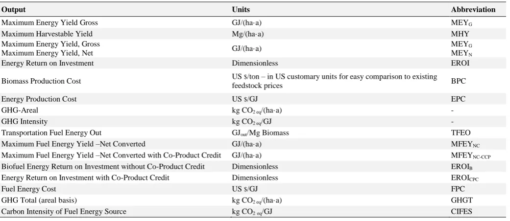
The approach of FEBEF is as follows: Compute an energy-limited carbon-capture by using growing-season solar energy inputs coupled with knowledge of the maximum photosynthetic rates of each feedstock. Similarly, compute a water-limited carbon-capture by using growing-season rainfall coupled with knowledge of the maximum WUE of each feedstock. De-rate both these carbon-capture estimates to account for multiple losses such as respiration and non-harvestable fraction, to estimate a light-limited and water-limited yield. Pick the lower of the two to estimate the biomass yield. The biomass yield is then used to calculate theoretical energy and biofuel yields. Break the cost of production and fuel conversion into fewer than a dozen line-items that are common across feedstocks, and use literature estimates to populate those cost estimates. Scale some of the line-items by yield (details below). Use an EIO-LCA approach to compute the embedded energy and GHG emissions from each cost line-item; sum both of these to find total embedded energy and GHG for each feedstock. With maximum yield, cost, energy input, and GHG emissions for each feedstock, key model outputs can be computed. These outputs are presented in Table S1.

S1. Background Assumptions and Calculations Worksheet

The BACC worksheets contain the following: BACC: (a) Text-color conventions used in the workbook. (b) Common conversion factors in named

cells (e.g., cell B12 is named kg per Mg and has a value of 1000). These conversions can be referred to by name elsewhere to reduce the incidence of hard-coding errors in the spreadsheet. (c) Molecular weights and densities of relevant materials. (d) Energy Contents and Thermodynamic Conversions. BACC-Crop: (a) Computations to convert literature data into ratios of root-exudate carbon to root stored carbon for Switchgrass and Miscanthus. (b) A listing of best-reported yields for each biomass type. Ideally these would be from identical environments in plots greater than 10 ha as the modeled case (central Iowa in this work), but this was only possible for corn; values for Switchgrass, Miscanthus, and algae were from more distant sites. (c) Theoretical limits on plant physiological parameters to allow an upper bound on the performance of the biomass. BACC-EconAsmp: (a) Economic assumptions including interest rates, utility prices, and inflation factors. (b) Raw data and linear regression of land rental costs vs. productivity data. (d) (f) (g) (i) BACC_EIO-LCA energy multiplier factors for perennial grass seeding. BACC-Fertilizer: (a) Fertilizer costs and pre-computations. (b) Fertilizer application rate crosscheck. BACC-Solar Solar and precipitation values. This includes raw meteorological data as well as data modified by the planting and harvesting dates listed in the Primary Assumptions worksheet.

S2. Cost vs. Yield Worksheet

The Cost vs. Yield worksheet (CvsY) scales line item production costs based upon predicted yields by assuming that some line items are yield-independent (i.e., scale factor n = 0), while others are linearly scaled with yield (n = 1). This binary segregation of costs is an oversimplification, but one which provides overall cost vs. scale responses is consistent with those reported for corn (data not shown). The yield-appropriate costs computed in the CvsY worksheet are used by the Primary Assumptions worksheet in the core cost model.

S3. Algae Cost Model Worksheet

The Algae Cost Model worksheet (ACM) contains the amortized capital, labor, irrigation, and direct energy cost calculations and free water evaporation calculation for three different algal production technologies in four different locations. The three different types of algal plants and the locations are ORP in Ames, IA, ORP in Tucumcari, NM, PBR in Phoenix, NM, and a coupled PBR-ORP system in Honolulu, HI. Each operation was assumed to have 100 ha production area. The amortized capital cost, labor,

Output Units Abbreviation

Maximum Energy Yield Gross GJ/(ha·a) MEYG

Maximum Harvestable Yield Mg/(ha·a) MHY

Maximum Energy Yield, Gross

Maximum Energy Yield, Net GJ/(ha·a)

MEYG MEYN

Energy Return on Investment Dimensionless EROI

Biomass Production Cost US $/ton – in US customary units for easy comparison to existing

feedstock prices BPC

Energy Production Cost US $/GJ EPC

GHG-Areal kg CO2 eq/(ha·a) -

GHG Intensity kg CO2 eq/GJ -

Transportation Fuel Energy Out GJout/Mg Biomass TFEO

Maximum Fuel Energy Yield –Net Converted GJ/(ha·a) MFEYNC

Maximum Fuel Energy Yield –Net Converted with Co-Product Credit GJ/(ha·a) MFEYNC-CCP

Biofuel Energy Return on Investment without Co-Product Credit Dimensionless EROIB

Energy Return on Investment with Co-Product Credit Dimensionless EROICPC

Fuel Energy Cost US $/GJ FPC

GHG Total (areal basis) kg CO2 eq/(ha·a) GHGT

CarbonIntensityofFuelEnergySource kg CO2eq/GJ CIFES

Table S1.

Conversion computations and key model outputs added to FEBEF.

(8)

and direct energy estimates for the production scenarios were based on literature reports, updated for inflation, and supplemented with engineering estimates when data was lacking. The irrigation costs were calculated from local pan evaporation data, growing season rainfall, and water rates. S3.1 ORP in Ames, IA

The ORP amortized capital costs were based on the 400 ha, 30 g/m2_/d production scenario using pure carbon dioxide outlined by Benemann and Oswald (1994). Capital costs for conversion equipment of algae oil to biodiesel, listed in the original publication, are excluded as a different source/method is used for fuel conversion capital cost estimates.

Line item capital costs were adjusted for inflation from 1994 dollars to 2008 dollars as shown in Equation 1.

𝐼𝑛𝑓𝑙𝑎𝑡𝑖𝑜𝑛 𝑎𝑑𝑗𝑢𝑠𝑡𝑒𝑑 𝑐𝑜𝑠𝑡 𝑓𝑜𝑟 𝑦𝑒𝑎𝑟 𝑦 = 𝐾𝑛𝑜𝑤𝑛 𝑐𝑜𝑠𝑡 𝑖𝑛 𝑦𝑒𝑎𝑟 𝑥 × (𝐼𝑛𝑓𝑙𝑎𝑐𝑡𝑖𝑜𝑛 𝑖𝑛𝑑𝑒𝑥 𝑓𝑎𝑐𝑡𝑜𝑟 𝑓𝑜𝑟 𝑦𝑒𝑎𝑟 𝑦

𝐼𝑛𝑓𝑙𝑎𝑡𝑖𝑜𝑛𝑖𝑛𝑑𝑒𝑥 𝑓𝑎𝑐𝑡𝑜𝑟𝑓𝑜𝑟 𝑦𝑒𝑎𝑟 𝑥)

(Eq. 1)

The total cost per line item for the 400 ha system was calculated. Using scale factors, assigned using engineering judgment to each line item, a total cost per line item for a 100 ha system is calculated as shown in Equation 2.

𝑃𝑟𝑒𝑑𝑖𝑐𝑡𝑒𝑑 𝐶𝑜𝑠𝑡 𝑜𝑓 𝑠𝑝𝑒𝑐′𝑑 𝑒𝑞𝑝 = 𝐾𝑛𝑜𝑤𝑛 𝐶𝑜𝑠𝑡 𝑜𝑓 𝑏𝑎𝑠𝑒𝑙𝑖𝑛𝑒 𝑒𝑞𝑝 ×

(𝑆𝑖𝑧𝑒 𝑜𝑓 𝑠𝑝𝑒𝑐′𝑑 𝑒𝑞𝑝

𝑆𝑖𝑧𝑒 𝑜𝑓 𝑏𝑎𝑠𝑒𝑙𝑖𝑛𝑒 𝑒𝑞𝑝)

𝑠𝑖𝑧𝑖𝑛𝑔 𝑒𝑥𝑝𝑜𝑛𝑒𝑛𝑡

(Eq. 2)

The sum of the line items gives a total capital investment. The yearly capital charges are calculated using the PMT function in Excel; the annual rate of return assumed in 10%, over a 20-year period, and total capital investment was the principal. The yearly capital charges (US $/a) is divided by 100 ha and converted to the reported estimate of amortized capital in US $/(acre.a).

The labor costs were based on Benemann and Oswald (1994) and were adjusted for inflation and seasonal labor needs. The baseline labor rate in US $/(ha·a) was adjusted for inflation as shown in Equation 1. The labor was prorated for the variation in the seasonal labor needs, as shown in Equation 3: 𝐿𝑎𝑏𝑜𝑟 𝑟𝑎𝑡𝑒 = 𝐼𝑛𝑓𝑙𝑎𝑡𝑖𝑜𝑛 𝐶𝑜𝑟𝑟𝑒𝑐𝑡𝑒𝑑 𝐿𝑎𝑏𝑜𝑟 𝑅𝑎𝑡𝑒 ×

(𝐹𝑟𝑎𝑐𝑡𝑖𝑜𝑛 𝑜𝑓 𝑌𝑒𝑎𝑟 𝐺𝑟𝑜𝑤𝑖𝑛𝑔 𝐴𝑙𝑔𝑎𝑒 + 𝐹𝑟𝑎𝑐𝑡𝑖𝑜𝑛 𝑜𝑓 𝑌𝑒𝑎𝑟 𝐼𝑑𝑙𝑒 ×

𝑃𝑒𝑟𝑠𝑜𝑛𝑛𝑒𝑙 𝑅𝑒𝑞𝑢𝑖𝑟𝑒𝑚𝑒𝑛𝑡𝑠 𝑖𝑛 𝑂𝑓𝑓 𝑆𝑒𝑎𝑠𝑜𝑛) (Eq. 3)

This prorated value was then scaled by system size, and adjusted for inflation.

The direct energy estimate was based on Benemann and Oswald (1994). The power requirements (kWh/(ha·a)) for mixing, centrifugation, water pumping, and other (nutrient pumping and building needs) were summed to find the total power requirement. The total power requirement (kWh/(ha·a)) was then multiplied by the local electricity rate (US $/kWh) (Energy Information Administration, 2010_{) to give a direct energy cost in (US $/(ha·a)), which was}

converted to US $/(acre.a) as reported in the Primary Assumptions worksheet. The irrigation costs for all of the algal production scenarios in the four different locations were estimated using the same method. We assumed that the evaporation of the free standing water at the different production plants was similar to lakes (Linacre, 2018), and that all of the evaporation occurred during the growing season. Local pan evaporation data (in/a) (Western Regional Climate Center, 1986_{) was manipulated by pan to lake evaporation factor, as}

shown in Equation 4_.

𝐿𝑎𝑘𝑒 𝑒𝑣𝑎𝑝𝑜𝑟𝑎𝑡𝑖𝑜𝑛 (𝑖𝑛

𝑎) = 𝑃𝑎𝑛 𝑒𝑣𝑎𝑝𝑜𝑟𝑎𝑡𝑖𝑜𝑛 ( 𝑖𝑛 𝑎) ×

𝑅𝑎𝑡𝑖𝑜 𝑜𝑓 𝐿𝑎𝑘𝑒 𝑡𝑜 𝑃𝑎𝑛 𝐸𝑣𝑎𝑝𝑜𝑟𝑎𝑡𝑖𝑜𝑛

(Eq. 4)

Then, daily evaporation rate was calculated as shown in Equation 5_.

𝐷𝑎𝑖𝑙𝑦 𝐸𝑣𝑎𝑝𝑜𝑟𝑎𝑡𝑖𝑜𝑛 (𝑐𝑚

𝑑) = 𝐿𝑎𝑘𝑒 𝑒𝑣𝑎𝑝𝑜𝑟𝑎𝑡𝑖𝑜𝑛 × (𝑐𝑚/𝑖𝑛)

𝑆𝑒𝑎𝑠𝑜𝑛 𝑙𝑒𝑛𝑔𝑡ℎ (𝑑) (Eq. 5)

The daily evaporation rate was converted to m3_{/d. The mass of water} evaporated is calculated as shown in Equation 6.

(Eq. 6) 𝑀𝑎𝑠𝑠 𝑤𝑎𝑡𝑒𝑟 𝑒𝑣𝑎𝑝𝑜𝑟𝑎𝑡𝑒𝑑 (𝑘𝑔

𝑑)

= 𝐷𝑎𝑖𝑙𝑦 𝑒𝑣𝑎𝑝𝑜𝑟𝑎𝑡𝑖𝑜𝑛 (𝑚

3

𝑑) × 𝐷𝑒𝑛𝑠𝑖𝑡𝑦 𝑜𝑓𝑤𝑎𝑡𝑒𝑟( 𝑘𝑔 𝑚3)

As a cross-check, an effective “WUE” was calculated for the algal scenarios as shown in Equation 7:

𝑊𝑈𝐸 =

(𝑀𝑎𝑥𝑖𝑚𝑢𝑚 𝐻𝑎𝑟𝑣𝑒𝑠𝑡𝑎𝑏𝑙𝑒 𝑌𝑖𝑒𝑙𝑑 (

𝑀𝑔 ℎ𝑎) 𝑆𝑒𝑎𝑠𝑜𝑛 𝐿𝑒𝑛𝑔𝑡ℎ−𝑑𝑎𝑦𝑠 ×

1000𝑘𝑔 𝑀𝑔 × 100ℎ𝑎)

𝑀𝑎𝑠𝑠 𝑤𝑎𝑡𝑒𝑟 𝑒𝑣𝑎𝑝𝑜𝑟𝑎𝑡𝑒𝑑 𝑘𝑔/𝑑

(Eq. 7)

Water use was corrected for local, annual precipitation as shown in Equation 8.

(Eq. 8)

〖𝑊𝑎𝑡𝑒𝑟 𝑈𝑠𝑒〗_(𝑝𝑟𝑒𝑐𝑖𝑝𝑖𝑡𝑎𝑡𝑖𝑜𝑛 𝑐𝑜𝑟𝑟𝑒𝑐𝑡𝑒𝑑) (𝑚/𝑠𝑒𝑎𝑠𝑜𝑛)

= [((𝐸𝑣𝑎𝑝. 𝑅𝑎𝑡𝑒(𝑐𝑚/𝑑) × 𝐺𝑟𝑜𝑤. 𝑆𝑒𝑎𝑠. 𝐿𝑒𝑛𝑔. (𝑑)) − (𝑃𝑟𝑒𝑐𝑖𝑝. (𝑐𝑚/𝑎)

× 𝐹𝑟𝑎𝑐. 𝑊𝑎𝑡𝑒𝑟 𝐴𝑣𝑎𝑖𝑙. 𝐷𝑢𝑟𝑖𝑛𝑔 𝐺𝑟𝑜𝑤. 𝑆𝑒𝑎𝑠. ))/(𝑐𝑚 𝑖𝑛)]

The volume of water evaporated over the whole free water area corrected for precipitation was calculated as shown in Equation 9.

(Eq. 9) 𝑊𝑎𝑡𝑒𝑟 𝑈𝑠𝑒𝑝𝑟𝑒𝑐𝑖𝑝.𝑐𝑜𝑟𝑟.(

𝑓𝑡3

𝑎)

= 𝑊𝑎𝑡𝑒𝑟 𝑈𝑠𝑒_{𝑝𝑟𝑒𝑐𝑖𝑝.𝑐𝑜𝑟𝑟.} ( 𝑚

𝑠𝑒𝑎𝑠𝑜𝑛) × 100 ℎ𝑎 × 𝑚2_{/ℎ𝑎 × 𝑓𝑡/𝑚}3

For the PBR in Phoenix, AZ, the calculation was adjusted to correct for the area of water baths, which was a fraction of the 100 ha.

Annual irrigation costs were calculated by multiplying the local industry water rates (US $/cubic feet) (Tucumcari, 2004; City of Phoenix Water Rates, 2010; City and County of Honolulu, 2015) by the Seasonal Water Use (cubic feet/season). The irrigation costs on an area basis are calculated as shown in Equation 10.

(Eq. 10) 𝐼𝑟𝑟𝑖𝑔𝑎𝑡𝑖𝑜𝑛 𝑐𝑜𝑠𝑡𝑠 (𝑈𝑆 $ ℎ𝑎⁄ ⁄ ) =𝑎 𝑌𝑒𝑎𝑟𝑙𝑦 𝐼𝑟𝑟𝑖𝑔𝑎𝑡𝑖𝑜𝑛 𝐶𝑜𝑠𝑡 (

𝑈𝑆 $ 𝑎)

100 ℎ𝑎

The irrigation costs (US $/(ha.a)) are converted to a US $/(acre.a) basis.

S3.2 Algae Harvesting

The harvesting of algae from the production reactors (ORPs or PBRs) included the capital costs for a primary settling followed by centrifugation. We assumed the centrifugation produced 15% solids from the ORP systems and 20% solids from the PBR systems. For the ORPs, we calculated the additional direct energy required to reach 20% solids, as shown in Equation 11.

Direct Energy_{algae slurry} = MHY × Hvap × MR% × (MC%/(1 − MC%)) (Eq. 11)

Where, Hvap is the heat of vaporization for water, MR% is the moisture (%) needed to remove to reach 10% solids, and MC% is the moisture content of the slurry exiting the centrifuge.

S3.3ORPinTucumcari, NM

The approach for computing amortized capital costs and labor costs was identical to that used for Ames, IA. The direct energy and irrigation costs used the same method but with electricity and water rates specific to Tucumcari, NM.

(9)

S3.4PBRinPhoenix, NM

The PBR amortized capital costs were based onGrima et al. (2003) report on commercial production of microalgae in PBRs. The basis of that study was a facility with a projected biomass productivity of 1.25 kg/m3_/d_{(approximately} 10.7 g/m2_{/d) in continuous culture. We included only the unit operations and} the associated costs needed for the cultivation of the algae and up through harvesting the algae.

The original line item capital costs included in the amortized capital estimate in 2001 dollars were adjusted for inflation as shown in Equation 1to 2008 dollars. The cost estimate was then scaled from the area of foot print (approximately 1 ha) of the PBR calculated from measurements given inGrima et al. (2003)to a 100 ha area using Equation 2.

The centrifugation costs provided by Grima et al. (2003) were replaced with a yield scaled centrifugation cost from Vadas et al. (2008) as shown in Equation 12. This allowed for consistency with the same unit operation across technologies.

(Eq. 12) 𝐶𝑒𝑛𝑡𝑟𝑖𝑓𝑢𝑔𝑎𝑡𝑖𝑜𝑛 𝑐𝑜𝑠𝑡𝑠𝑡𝑒𝑐ℎ (𝑈𝑆 𝑈𝑆 $)

= (𝑀𝑎𝑥𝑖𝑚𝑢𝑚 𝐻𝑎𝑟𝑣𝑒𝑠𝑡𝑎𝑏𝑙𝑒 𝑌𝑖𝑒𝑙𝑑𝑡𝑒𝑐ℎ 𝑀𝑎𝑥𝑖𝑚𝑢𝑚 𝐻𝑎𝑟𝑣𝑒𝑠𝑡𝑎𝑏𝑙𝑒 𝑌𝑖𝑒𝑙𝑑𝑂𝑃𝑅

)

× 𝐶𝑒𝑛𝑡𝑟𝑖𝑓𝑢𝑔𝑎𝑡𝑖𝑜𝑛 𝐶𝑜𝑠𝑡𝑠_𝑂𝑃𝑅

The total capital cost was the summationof the scaled costs. The yearly capital charge was computed using an annual rate of return at 10% over a 20-yearperiod. The yearly capital charge (US $/a) was divided by 100 ha and converted to the reported estimate of amortized capital in US $/(acre.a).

The labor costs were based onGrima et al. (2003), adjusted for inflation and scale. These labor costs were prorated based on the growing season length (fewer workers off season).

The direct energy estimate was also based on the Grima et al. (2003), using local electrical rates(Energy Information Administration, 2010)in Phoenix, AZmand converted to US $/(acre.a)for the direct energy costs.

S3.5Coupled PBR-ORP system inHonolulu, HI

The Coupled PBR-ORP amortized capital costs based primarily onHuntley and Redalje (2007) which reported the general specifications of the Aquasearch (now HP petroleum) coupled production systems for photosynthetic microbes. Biomass production was estimated at 10.2 g/m2_/d_{for the PBR and 15.1 g/m}2_/d for the ORPs. The authors of Huntley and Redalje (2007) relied on the

Benemann and Oswald (1994) techno-economic analysis (adjusted for inflation) for capital costs for the ORPs, and on Hallenbeck and Benemann (2002) for PBRcost estimates. We included only the unitoperations and the associated costs needed for the cultivation of the algae and up through harvesting the algae.

Capital costs were adjusted for inflation and scaled. Centrifugation costs were calculated as outlined above using Equation 11. The yearly capital charge was computed using an annual rate of return at 10% over a 20-yearperiod. The yearly capital charge (US $/a) was divided by 100 ha and converted to the reported estimate of amortized capital in US $/(acre.a).

The labor costs were calculated based on both the previous PBR and ORP labor estimates. The percentage areasof the PBR and ORP unit operations of the total operational area werecalculated. The labor costs for the coupled system were estimated by distributing the percentagearea with the labor costs, as shown in Equation 13.

𝐿𝑎𝑏𝑜𝑟 𝑐𝑜𝑠𝑡𝑃𝐵𝑅−𝑂𝑅𝑃= 𝑃𝐵𝑅 𝑎𝑟𝑒𝑎 % × 𝐿𝑎𝑏𝑜𝑟 𝐶𝑜𝑠𝑡𝑃𝐵𝑅+ 𝑂𝑅𝑃 𝑎𝑟𝑒𝑎 % ×

𝐿𝑎𝑏𝑜𝑟 𝐶𝑜𝑠𝑡𝑂𝑅𝑃

(Eq. 13)

These labor costs were prorated based on the growing season length (fewer workers off season).

The direct energy costs were calculated fromthe previous PBR and ORP power estimates. The power needs for the coupled system were estimated by distributing the percentage area with the direct energy estimates, as shown in Equation 14.

𝑃𝑜𝑤𝑒𝑟 𝑅𝑒𝑞𝑢𝑖𝑟𝑒𝑚𝑒𝑛𝑡 𝑃𝐵𝑅−𝑂𝑅𝑃 (𝑘𝑊ℎ_{ℎ𝑎·𝑎}) = 𝑃𝐵𝑅 𝑎𝑟𝑒𝑎 % ×

𝑃𝑜𝑤𝑒𝑟 𝑅𝑒𝑞𝑢𝑖𝑟𝑒𝑚𝑒𝑛𝑡_𝑃𝐵𝑅+ 𝑂𝑅𝑃 𝑎𝑟𝑒𝑎 % × 𝑃𝑜𝑤𝑒𝑟 𝑅𝑒𝑞𝑢𝑖𝑟𝑒𝑚𝑒𝑛𝑡_𝑂𝑅𝑃

(Eq. 14)

This estimated power requirement was then multiplied by the electricity rates in HI (Energy Information Administration, 2010)to calculatethe direct energy cost in US $/(ha·a) and then converted to US $/(acre.a).

S4. Primary Assumptions Worksheet

The Primary Assumptions worksheet (PA tab) compiled literature-based measurements and assumptions about climate, plant growth, production costs, energy requirements, GHG emissions, water use, and eutrophication potential. In some cases, data came directly from literature sources, while in others, it was based on computations in the supporting worksheets that have been previously described. In all cases, the data for each feedstock was organized in a single column. Details of the contents of the Primary Assumptions worksheet follow:

S4.1 Location-Specific Climatic Assumptions

Annual average solar irradiation (W/m2_{) (}_{Marion and Wilcox, 1995}_), fraction of solar radiation in as photosynthetically available radiation (PAR) (Bolton and Hall, 1991), annual total rainfall (http://www.weatherbase.com/weather/state.php3?c=US&refer), planting date, and harvesting date (Neild and Newman, 1990; Wolf and Fiske, 1995; Chisti, 2007) are the four fundamental assumptions entered into the climate section of the model. These fundamental assumptions are used to compute growing season length, fraction of solar available during growing season, and fraction of water available during growing season. To find the latter two items, intermediate calculations are conducted in the Background Assumptions and Calculations worksheet.

S4.2Crop Physiological Assumptions

Crop performance data and cost estimates are based on literature values without extrapolations based on future technological advances.

Literature Reported RUEvalues

RUEis a measure of biomass accumulation given PAR. Instantaneous RUEs(g of biomass/MJ of PAR) were estimated for C4 plants fromNobel (1991) and for algae from Melis (1998) by converting gas evolved (CO2or O2) and photon flux density converted to anRUE.

RUE actual to RUE Theoretical MaximumRatio(RUER)

The maximum theoretical RUEis assumed to be 30% on PAR basis (Bolton and Hall, 1991). The ratio of the crops’ actual RUE to the RUE theoretical maximum is calculated by FEBEF, as shown below in Equation 15, where RSR is the Root: Shoot Ratio at harvest:

𝑅𝑈𝐸𝑅 = (𝑅𝑈𝐸𝑎𝑐𝑡𝑢𝑎𝑙(

𝑔 𝑏𝑖𝑜𝑚𝑎𝑠𝑠

𝑀𝐽 ) × 𝐵𝑖𝑜𝑚𝑎𝑠𝑠 𝐸𝑛𝑒𝑟𝑔𝑦 𝐶𝑜𝑛𝑡𝑒𝑛𝑡( 𝑀𝐽

𝑔)

𝑅𝑈𝐸𝑀𝑎𝑥(𝑔 𝑏𝑖𝑜𝑚𝑎𝑠𝑠𝑀𝐽 )

) × (1 + 𝑅𝑆𝑅)

(Eq. 15)

Literature Reported WUE Values

The instantaneous WUEvalues for the terrestrial crops, defined as the ratio of biomass accumulated to crop water transpired, was experimentally determined inRochette et al. (1996), and these values were used in the model. The term WUE is normally not used when referring to aquatic plants. However, if one pictures the entire culture system as a giant “leaf,” an effective WUE can be computed. The WUE of the algal crop was computed as the growing season evaporation from pond divided by the algal biomass produced. The transpiration calculations were previously described in Equation 7.

(10)

WUE actual to WUE Theoretical MaximumRatio(WUER)

The theoretical maximum WUE was estimated based on an assumed leaf temperature, ambient relative humidity, maximum net photosynthetic rate, and water vapor flux for a typical Iowa crop. The calculations were shown in the Background Assumptions Worksheet. The value estimated and used in the model was 0.02 kg biomass/kg water.

Respiration Loss of Fixed C (RLC) -Growing Seasonal Average (GSA)

Stored chemical energy is lost viarespiration whichsupports physiological needs including transportation and translocation of nutrients, protein and lipid synthesis, and cellulose synthesis. While the respiration losses are dependent on the needs the plant, we estimated growing seasonal average(Taylor etal., 1998).

Root: Shoot Ratio @ harvest (RSR)

This experimentally determined value is the ratio of dry belowground structural root biomass to dry aboveground biomass. Literature-reported values for the different terrestrial cropswere used(Kiniryet al., 1999; Kahle et al., 2001; Bonifas et al., 2005).

C to soil organisms / C in root (GSA) CSORR

For terrestrial crops, a fraction of the carbon captured is transferred to the soil in the form of root turnover, root cap mucigel,and organic exudates(Amos and Walters, 2006).Literature-reported values for net rhizodeposited carbon for the different terrestrial cropswere converted to a root basis ratio(Frank et al., 2004; Wanga et al., 2005; Amos and Walters, 2006). Those conversion calculations were done in the Background Assumptions worksheet.

Fraction of Stover Collected

In light of equipment collection limitations and sustainable collection guidelines, the fraction of corn stover collected was assumed to be 60% (Glassner et al., 1998).

Harvestable Fraction of Above Ground Biomass (hfAGB )

Thisfactor accounted for mechanical limitations of the production harvest systems. Literature-reported values for the different terrestrial crops and algae were used(El Bassam and Huisman, 2001; Vogel, 2002; Huntley and Redalje, 2007; Johnson, 2007).

Harvestable Fraction of Total Biomass (hfTB )

This factor accounted for the belowground biomass and was calculated in FEBEF by Equation 16, as shown below:

ℎ𝑓𝑇𝐵=

𝐻𝑎𝑟𝑣𝑒𝑠𝑡 𝐼𝑛𝑑𝑒𝑥 1+𝑅𝑆𝑅

(Eq. 16)

Harvestable Fraction of Total Fixed Carbohydrate (hfTFC )

This term represented the harvestable portion of carbon captured by the plant over the season. FEBEF calculated this factor by Equation 17:

ℎ𝑓𝑇𝐹𝐶=

ℎ𝑓𝐴𝐺𝐵

(1+𝑅𝑆𝑅+𝑅𝑆𝑅×(𝐶𝑆𝑂𝑅𝑅))×(1−𝑅𝐿𝐶)

(Eq. 17)

Biomass Energy Content (BEC)

The higher heating values of the crops were experimentally determined and reported in(Beale and Long, 1995; McLaughlin, 1996; Hase et al., 2000; Brown Robert, 2003; Pordesimo et al., 2005)and were utilized in the model in units of MJ/kg.

Biomass Moisture Content @ Harvest

This factor was aliterature based estimate for the amount of moisture remaining in the biomass following harvesting.

Additional Moisture Removal Needed

This is an estimate of the amount of moisture needed to be removed from the biomass to allow for storage and/or fuel processing.

Direct Energy for Moisture Removal

This calculation is described earlier in Equation 11to estimate the additional direct energy requiredto reach 10% solidsfor the algae systems.

Technological Improvement in Energy Reduction for Dewatering

This value is an estimate that attempts to credit algal production technologies with harvesting developments that result in lower direct energy costs to meet desired moisture content levels.

Direct Energy Cost for Moisture Removal

This calculation estimates the direct energy cost needed to meet desired moisture content using natural gas to remove the moisture while also crediting for technological improvements to harvesting as shown in Equation 18:

𝐷𝐸𝐶 =

(Direct Energyalgae slurry×1000kWhMJ× GJ

1000MJ×Natural Gas Cost US $

kWh)×(1−Technological Improvemnt for Dewatering) (2.471acres_ha)

(Eq. 18)

S4.3 Crop-Cost Components

Land rental cost was assumed to be proportional to biomass harvest. A linear regression model was developed from the reported cash rental rates and typical corn yields for high, medium, and low quality cropland (Edwards, 2009). Arguments have been made that feedstocks other than corn, including algae, for biofuels could be grown on marginal land and avoid competing for high value land, and therefore lower production costs. However, cash rental rates typically reflect average yields and we assume that this trend would apply to all bioenergy crops. The application of this model not only indirectly reflects nutrient removal from soil given yields for the terrestrial crops but also that higher output generates a surplus that is likely to be appropriated by the land owner in the charge of rent.

Amortized capital, labor, direct energy, biological capital, and lime and biocide costs for the terrestrial production scenarios were estimated by taking baseline values and either as is, or scaled to yield. Amortized capital costs were assumed independent of yield. While this is not true in the extremes –greater yields could conceivably require larger machinery –we argue it is a good first approximation. In contrast, labor costs, direct energy costs,and biological capital are assumed proportional to yield. Lime and biocides (pesticides, herbicides) are assumed to be independent of yield. Original production cost values were gleaned fromVadas et al. (2008) and

Smeets et al. (2009). Chemical costs, while proportional to yield, were computed based on the N, P, and K content of the harvested biomass (Wallace, 1923; Zelibor et al., 1998; Lemus et al., 2002; Tokuşoglu and

Üunal, 2003; Hoskinson et al., 2007; Johnson et al., 2007; Monti et al., 2008)and upon an assumption of the fraction of chemicals in the harvested biomass compared to the fraction applied. Irrigation costs for algal scenarios came from the algae cost model worksheet.

S4.4 Single Pass Corn Grain and Stover Harvesting Assessment

Based on Turhollow and Sokhansanj (2007) whichassumes that 2/3 (10% more than for double pass) of the corn stover can be harvested in a single pass along with corn grain, with a reduced combine harvesting efficiency of 55% from 70%, the following estimates were made