Predict VLSI Circuit Reliability Risks Using Neural Network

(1)

Predict VLSI Circuit Reliability Risks Using

Neural Network

Wei-Ting Kary Chien, Randy Kang

*

_{, Howking Sii, Ming Li}

Qualify and Reliability Center, Semiconductor Manufacturing International (Shanghai) Corp. Shanghai, China *Corresponding Author: [email protected]

Abstract

This paper describes the challenges faced in predicting the reliability of very large scale integration (VLSI) circuits. Currently, lots of trial-and-errors are still needed for the parameters selected to develop a neural network prediction model, whose result is with a great deal of uncertainty. The objective of this paper is to provide a novel and practical approach to design a reliability prediction model using neural network. We propose a seven-step procedure to formulate an optimal neural network design and explain it in details using a case study on semiconductor reliability. We combine reliability test characteristics (e.g., early failures) with statistical methods such as regression and design of experiment (DOE) for this optimal neural network model and get comparably small prediction errors. Following our proposed approach, analysts can develop effective designs with higher prediction accuracy. We further introduce an operation flow to maximize the benefits from the obtained optimal prediction model by earlier nonconformance detection and faster lot dispositions, which are reported in the case study on successfully implementing our methodology to predict inter metal dielectric (IMD) reliability risks. Our proposed approach can be easily applied on many other fields like yield prediction.

Keywords

Neural Network, Prediction; IMD Reliability, DOE; Correlation Analysis, Linear Regression

1. Introduction

Reliability is one of the important factors affecting the development and profitability of semiconductor manufacturing. Conventionally, semiconductor reliability can be estimated from the accelerated stress tests, which include two major categories in semiconductor manufacturing: process and product reliability tests. For product reliability tests, like High Temperature Operating Life (HTOL) and Temperature Humidity with Bias (THB), we test the samples after assembly; these tests are the

traditional ways to judge the final reliability performance and are time consuming. There are wafer- and package-level tests for process reliability, which test specially designed test structures (instead of the real products like those for most product reliability tests) and provide more timely information on reliability risks.[1] Especially for wafer-level process reliability tests, since we directly test wafers, we can quickly obtain reliability test results to assess risks. Therefore, the wafer-level process reliability is widely used as an in-line test to early detect nonconformance.[2] In this paper, we hence focus on the in-line wafer-level process reliability tests which are essential to semiconductor manufacturers’ profitability and success.

Traditionally, we can only assess reliability risks after tests, which may be either in-line or end-of-line.[3] After accumulating sufficient test data, we can formulate baseline records for, e.g., the Ea. of metal Electro-Migration (EM)[4], the current degradation of a device, and the breakdown voltage (Vbd) of a dielectric layer. The baseline records could be further refined after a failure occurs and the corresponding improvement actions are taken. Moreover, we can define safe margins based on the variations gathered from all previous tests and develop suitable test-to-target methodologies to early detect process drifts.[5] However, to assess reliability risks at a much earlier time, it will be very effective if we have a reliability prediction model which is only based on available production parameters (and without reliability tests).

(2)

determining the number of neurons in the hidden layer, collecting sufficient data sets, and best allocating the data sets for training, validations, and tests. All these will be discussed in depth in this paper.

To elucidate our proposed approach and the settings of the neuron network model, we report a case study on assessing IMD reliability risk. IMD is a dielectric layer used to electrically separate metal interconnects in an Integrated Circuit (IC). With the continuous scaling of IC’s, the Ramp-Voltage (Vramp) of IMD test is one of the important reliability assessments to assure IMD robustness.[8] Using neuron network to construct a non-linear prediction model is an ideal approach to fit the various manufacturing conditions. We use DOE and regression methods to improve prediction accuracy. A test flow is provided to meet practical needs and to closely link the neuron network prediction model and the in-line reliability tests to confirm failures, dispose nonconforming material, and refine the neuron network model. From the actual production in a long term, we find the proposed approach and the flow do lead to tremendous cost reduction because of the more accurate predictions and the earlier detections. Furthermore, our proposed approach can also be extended to predict yield.

This paper is organized as follows. In Section 2, the architecture of neuron network is briefly introduced; and we also describe the capability of neuron network to develop and adjust its own model to match the complexity of the historical input data for failure prediction. Section 3 presents our approach that uses the seven-step working flow to design an optimized neuron network prediction model. A real case study is reported on IMD reliability prediction. Finally, we conclude the paper in Section 4.

2. Neural Network

Neuron network, inspired by biological brain functions, is a simplified mathematical model to define a function or a distribution. Compared to conventional analysis software which produces data for people to make decisions, neuron network examines data, learns from itself, and makes its own decisions.[9] In technical terms, neuron network performs a non-linear mapping from inputs to outputs. This is a type of non-linear processing system that can map most nonlinear functions, essentially universal function approximators.[10] As such a highly flexible function approximator, it is powerful for pattern recognition, classification, and prediction. It has wide applications on various fields and industries.[11]

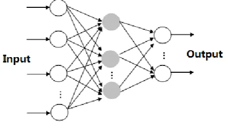
The architecture of a general neuron network with three layers, i.e., an input, an output, and a hidden layer, is shown in Figure 1, where all input factors are placed in the input layer and response parameters are placed in the output layer. In the hidden layer, there are several neurons connecting both input and ouput layers. This makes the function transformation with defined mathematical arithmetic. The coefficients of arithmetic can be trained and adjusted by all

information from the input layer. After comparing the output predictions with the actual results, neuron network can feed forword the information to model and adjust the coefficient of arithmetic till the prediction error from the real results is acceptable. So the configuration of the hidden layers is very improtant for setting an neuron network model. In terms of the number of hidden layers, a three layer neuron network model, i.e., the neuron network model with only one hidden layer, is adequate to most mathematical functions.[12] Therefore, to be suitable for the most situations, we limit our neuron network to be 3-layer for simplicity.

Figure 1. Structure of a three layers of neuron network

There are two indices we can use to evaluate the fitting of the neuron network model. One is Mean Square Error (MSE), as in (1), which is a risk function, corresponding to the expected value of the squared error loss or quadratic loss. The smaller the MSE, the better the fitting of the neuron network model.

∑

=

−

=

n

i i i

Y

n

MSE

1

2

)

ˆ

(

1

(1)

i

Y

: the real value of reliability test

i

Y

ˆ

: the prediction value of reliability test n: the total count of test group

The other index is R2_{, which is the coefficient of}

determination. It indicates how well the data points fit a statistical model.

tot res

SS

R

2

=

1 −

(2)

∑

=

−

=

n

i i tot

Y

SS

1

2

)

ˆ

[image:2.595.314.548.224.351.2]

(3)

∑

=

−

=

n

i i i

res

Y

SS

1

2

)

ˆ

(

(4)

Y

: the average of reliability test result

tot

SS

: the total sum of squares

res

SS

: the sum of squares of residuals

The limitations of neuron network model are that the development process requires tedious experiments with trials and errors, intensive computation, and proper selection of neuron network architectures. The neuron network prediction results are sensitive to the selection of learning input parameters. The development and interpretation of neuron network also require a great deal of expertise from users. However, these problems can all be minimized by our proposed approach, which will be introduced in the next section.

[image:3.595.313.549.298.701.2]

3. Reliability Prediction Working Flow

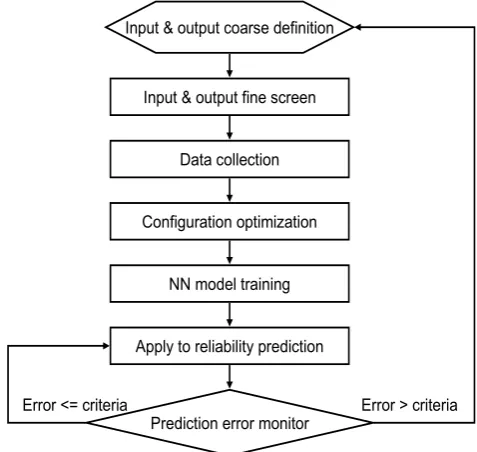
We propose a seven-step (including 6 designs and one monitor step) to formulate an optimal neuron network model as presented in Figure 2. The procedure is usually not a single-pass, but requires several repetitions on neuron network model training and input & output fine screen step.

Figure 2. Flow of using neuron network model to predict reliability risks

3.1. Input & Output Initial Selection

This step is an initial selection because the input and output factors can be selected to express the process characteristics. Successfully designing a neuron network

prediction model depends on a clear understanding of the problem and what input and output parameters are to be used. At this point in the initial selection step, the concern is on the raw data from which a variety of parameters will be collected and developed, because these parameters will form the inputs of the neuron network model for training. In short, input data should cover all key factors that are related with IMD process in the case study. Moreover, the past IMD reliability failure lesson-learnt cases’ root-cause parameters should also be considered as key input factors to improve forecasting performance. For example, the Vramp test early fail (EF) results should be selected as key factors of input and output for neuron network model training. Figure 3(A) shows typical Weibull plot and Figure 3(B) shows typical EF IV curves of IMD Vramp test. The products with EF indicate that reliability risk is high. In our case, total 124 data sets are collected and 11 of them have EF. This includes about 2 years of reliability WLR monitoring history data.

A

B

Figure 3. Part A: A typical IMD Vramp of Weibull plot with two early fail. X-axis is value of breakdown voltage; Y-axis is the CDF% (Cumulative Distribution Function). Part B: IMD Vramp Early Fail sample IV curve (Pink) and Vramp pass sample IV curve (Black). X-axis is stress voltage; Y-axis is Leakage current.

Input & output coarse definition

Input & output fine screen

Configuration optimization

NN model training

Apply to reliability prediction

Prediction error monitor Data collection

[image:3.595.57.296.435.661.2]

(4)

To properly select input parameters from the many candidates such as the power/ gas flow/ pressure of a processing tool, the inline measurements, and the electrical test results, we must have process, product and equipment engineers involved in the first screening. After consulting responsible owners, we select wafer thickness, Critical Dimension (CD), gas flow in IMD process tools, Radio Frequency (RF) power, temperature and process waiting time as inputs. At the initial selection stage, we include all related parameters regardless their physical, chemical, and technical meaning to avoid missing important ones.

At the output definition stage, we need define the problems and identify indices to best reflect the requirements. The guidelines to define output(s) are listed below.

a) The input and output parameters are required to be collected by wafer, by lot, or by die correspondingly to represent real parameter for higher prediction

accuracy.

b) It has more information for using raw data (e.g., film thickness) than the statistics (e.g., the average film thickness) for higher prediction accuracy.

c) When we had to use statistics instead of raw data, because of guideline #a, we should use meaningful statistics rather than some specially defined values. For example, we use mean & standard deviation for normally distributed data; for data following a Weibull distribution, we should use shape and scale parameter as much as possible.

d) Use min. output factor for better prediction accuracy. In our case, the output factor is each lot’s Vbd_0.1% from the Vramp stress test, whose spec is, e.g., > 3.2MV/cm.

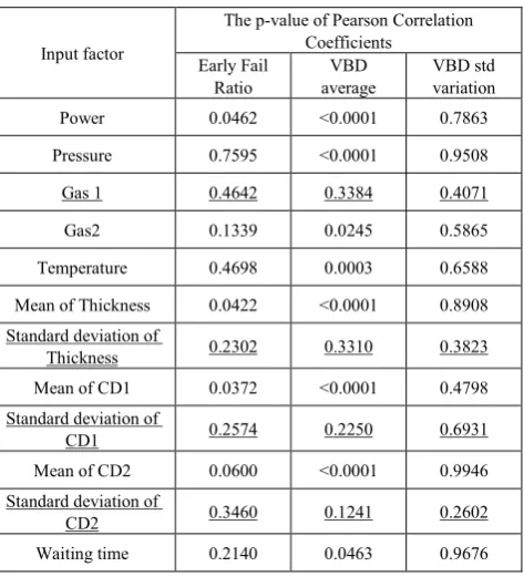
Table 1. Factor screen with linear regression

Input factor

The p-value of Pearson Correlation Coefficients

Early Fail

Ratio average VBD VBD std variation

Power 0.0462 <0.0001 0.7863

Pressure 0.7595 <0.0001 0.9508

Gas 1 0.4642 0.3384 0.4071

Gas2 0.1339 0.0245 0.5865

Temperature 0.4698 0.0003 0.6588

Mean of Thickness 0.0422 <0.0001 0.8908

Standard deviation of

Thickness 0.2302 0.3310 0.3823

Mean of CD1 0.0372 <0.0001 0.4798

CD1 0.2574 0.2250 0.6931

Mean of CD2 0.0600 <0.0001 0.9946

CD2 0.3460 0.1241 0.2602

Waiting time 0.2140 0.0463 0.9676

3.2. Refined Input & Output Selection

This step is critical to ensure prediction accuracy. Using all initially defined parameters in model fitting may be confounded by irrespective parameters. We suggest using factor screening to identify strongly correlated parameters. Many screening methods could be considered, such as linear regression, non-linear regression, stepwise regression and decision tree. For simplicity, we use linear regression and screen out eight out of twelve input parameters. As shown in Table 1, we use Pearson correlation to justify whether the input is significant to the output. For a p-value less than 0.05, it indicates the parameter is statistically significant to the output. From Table 1, we find four parameters (Gas 1, Standard deviation of Thickness, Standard deviation of CD1, and Standard deviation of CD2), which are underlined, are not significantly correlated to the outputs.

[image:4.595.311.553.301.403.2]

By doing this, as shown in Table 2, we reduce ~30% prediction error in the final prediction results.

Table 2. Prediction error comparison by refined selection

Item Early Fail _Ratio _averageVBD VBD std _variation

A: Prediction Error

(Before refine selection) 2.21% 6.0149 1.9385

B: Prediction Error

(After refine selection) 1.48% 3.9029 1.3665

Reduction ratio:

(A-B)/A 33% 35% 30%

3.3. Data Collection

The data used to train the network also play critical roles on the model predictability. The data must incorporate as much knowledge on the process as possible so the neuron network model can learn the best from the historic records and is able to provide more accurate prediction. As a rule of thumb, the data must cover the full range of inputs in which the network will be used. That is, the neuron network will not be able to accurately extrapolate itself beyond this range.[13] Data need to be preprocessed (i.e., normalized or standardized) and divided into subsets before being used to train the network. Our guidelines for data collection are summarized below.

a) Data must well represent the population.

b) The range of data needs cover all possible values of the parameter.

c) Both input and output need be normalized or standardized to [0, 1].

d) Both input and output data should be at the same grouping level like by lot, by wafer, or by die data.

3.4. Configuration Optimization

[image:4.595.62.299.468.729.2]

(5)

the most critical ones to prediction accuracy are the data set ratios of training/ validation/ test and the number of hidden neurons. One of our innovations is to apply statistical DOE to optimize neuron network configurations for a minimal MSE and a maximal R-square response.

Since optimal design uses less experimental runs to predict the response surface considering the interactions and quadratic effects, we use such DOE scenario to optimize the configurations. Less experimental runs mean a shorter test time, which is the major benefit to manufacturing industries. Using DOE, we can arrange a uniform and dispersive experiment at whole design space, and the result of DOE can be analyzed with regression or ANOVA model to well predict result. We further employ statistical analysis methods like regression and Analysis of Variation (ANOVA) to assist decision making.

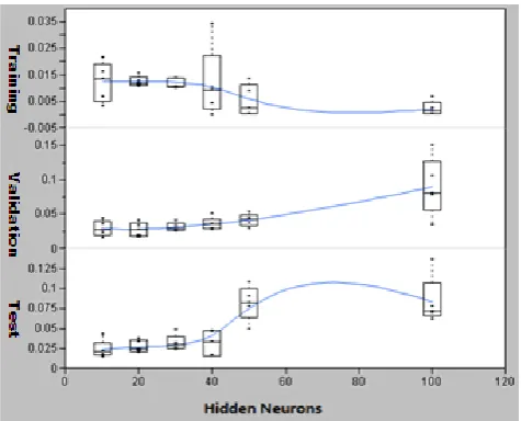
[image:5.595.314.552.219.411.2]

As mentioned, the factors to be decided are neurons in hidden layers, validation data set ratio, and test data set ratio. Because the sum of the data set ratio for training, validation, and test is 100%, we only need consider two of them in DOE as shown in Table 3 and 4, which gives the range of the most critical parameters. As in Figure 4, we tested the effect of hidden nuerons on MSE, and found, when hidden nuerons were larger than 50, both mean and variation of MSE increase significantly with validation and test data set ratios. The validation and test data set ratios are used to predict future data, which are our focuses. From Figure 4, we decide the hidden neurons to be less than 50 after balancing these three groups of data (i.e., Training, Validation, and Test).

Table 3. The major settings of the DOE input

Input Factor Levels Value

Hidden Neurons 4 10 ~ 50

Validation data ratio (%) 3 10 ~ 30

Test data ratio (%) 3 10 ~ 30

Table 4. The output response of DOE

Output Response Purpose Goal

MSE Minimum <0.02

R-square Maximum >90%

From the eight experimental runs designed by the optimal DOE, we obtain the prediction profiler plots, as shown in Figure 5, which shows the optimal neuron network model could be derived when both validation and test data set ratios are 10% (i.e., the training data set ratio is 80%) and the number of hidden neurons is 50. The predicted MSE can achieve 0.0154 with 95% confidence range [0.0126, 0.0181]; this is better than the goal defined. The R-square is 0.946202 and its lower 95% bound, 0.93636, is also higher than the pre-specified level (0.90).

From Figure 5, when increasing hidden neurons and

reducing validation and test data set ratio, we can improve the model with a smaller MSE and a larger R-square. In this IMD reliability risk prediction, we finalize the configuration of neuron network model,which uses 10%, 10% and 50 as validation data set ratio, test data set ratio and hidden neurons, respectivly. But as shown in Figure 5, if we have more test data, reducing the percentage of validation and test data set ratio may further improve the R-square and MSE.

[image:5.595.59.299.444.613.2]

We find DOE is an effective method to quickly configuire neuron network and to clearly show the trend and interaction among critical parameters.

Figure 4. The MSE with different numbers of hidden neurons. X-axis is different Hidden Neurons number; Y-axis is MSE value in different group.

Figure 5. Prediction profiler for DOE result. X-axis is different factors in experiement; Y-axis is MSE and R value

3.5. Neuron Network Model Training

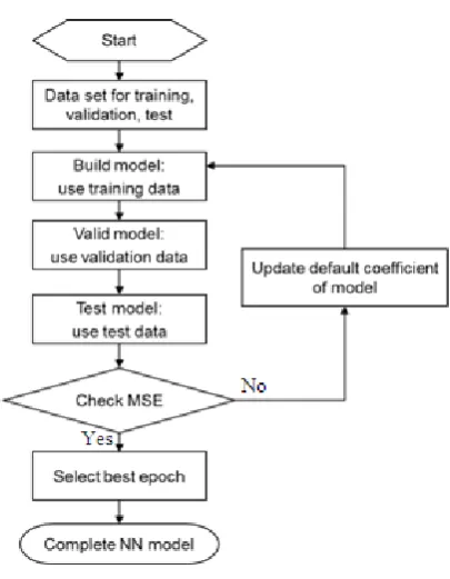
[image:5.595.312.552.457.613.2]

(6)

Figure 6. Neuron network model setup flow

Firstly, the system uses training set to build the initial neuron network model with default coefficients. Then, the initial model is used to predict and calculate MSE by validation model. A check function is used to verify whether the MSE is small enough to the case. If it is not acceptable, the system can save the current coefficients and start one new epoch to repeat training and validation till the MSE is small enough or reaches the maximum epoch number. The maximun epoch number is set to protect the system into infinite loop. When it happened, you need recheck the coefficients, inputs and output(s).

To aviod over fitting, the system can select the best epoch from all MSE data. A model which has been overfit will generally have poor predictive performance, as it can exaggerate minor fluctuations in the data.[14] As shown in Figure 7, this case runs 6 epochs, and the MSE of validation set is minimal in epoch 2. Thus, epoch 2 is selected as the best epoch and the coefficients are used in the final model. Because the model is built by training and validation sets, the test set is used to demo the situation when the model is applied in an actual environment.

Next, we use the best conditions from DOE to train and validate the final neuron network model. Figure 8(A, B, C) are the regressions of training, validation, and test, respectively, between the actual and prediction results. The regressions of all test data are in Figure 8(D). These plots can show if the prediction results are well fitting the actual values. The Y axis is the prediction result for output, and the X axis is the acutal result for target. So, if the points distribute near the liner Y=X, it means the good fitting of neuron network model. We can use R-square to judge the performance. In our test, finally, the MSE of IMD reliablity prediction model can

[image:6.595.79.282.78.339.2]

reach 0.0112 and R-square is 96%.

[image:6.595.316.548.94.285.2]

Figure 7. Selection for the best epoch. X-axis is epoch number; Y-axis is MSE value

Figure. 8. Prediction results vs. target. Part A: training data set; Part B: validation data set; Part C: test data set; Part D: all data, including training, validation and test data set. X-axis is real output value; Y-axis is predicted output value.

There is a guidance on model training: the test and validation data fittings need be close to training data. For example, the R-square gap between training and validation (or test) is not larger than +/-5%. This can make the model be easily fitting for more data in practice. After completing the model training, this neuron network model can be saved and used for real-time monitoring.

[image:6.595.315.549.326.581.2]

(7)

The criteria of judgment need be defined based on prediction errors and applications. For example, in this case, from neuron network prediction results, we have the prediction error of 0.3856 for one sigma, and the 95% probability range is thus 0.6339. The value of 3.2 MV/cm is the physical failure criteria for IMD reliability. Then we can define the 95% confidence prediction criteria is (3.2-0.6339 = 2.57 MV/cm, 3.2+0.6339 = 3.84 MV/cm). When real time prediction value is larger than 3.84 MV/cm, we can judge this lot’s IMD reliability will pass. Vice versa, when the real time prediction value is less than 2.57 MV/cm, we can judge this lot’s IMD reliability will fail. And this judgment’s confidence level is no less than 95%. But, if the prediction value is not in the range of (2.57~3.84 MV/cm), we cannot make the judgment just base on the prediction results, because the confidence of making this judgment is less than 95%. We call this an uncertain area, and more test data are required to verify the prediction results before making the final judgment.

We test this prediction model with 124 samples. There are 10 samples predicted in uncertain range, i.e., about 92% of the samples can be made prediction judgment. And comparing the prediction results with the real reliability test results, the successful ratio of prediction is 100%, i.e., this neuron network model makes a successful prediction for all other 114 samples. The results are really encouraging. This means we can forecast the reliability failure of wafers before they finish the manufactory processes. It is great useful to early alarm process abnormality, and engineers can quickly take actions to prevent larger impact and cost is thus saved.

3.7. Implementation of Neuron Network Model for Reliability Risk Prediction in IC Foundry

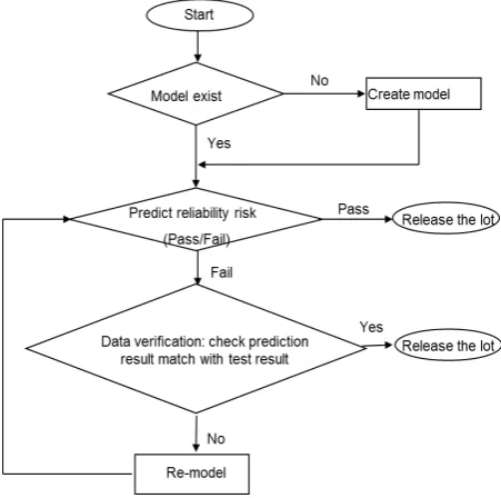
Neuron network model can be implemented for reliability risk prediction in IC foundry. A flow for such purpose is in Figure 9. The starting point can be from all Wafer Level Reliability Control (WLRC)[3] monitoring lot and excursion event lot that are related to IMD process. This can ensure the neuron network model be adapted to the real time application. Moreover, a regular review and monitor for the efficiency of the model is required. We set the prediction successful ratio as 95%. If the long term data, e.g., quarterly or semi-annually, show the successful ratio is less than 95%, a neuron network re-modeling flow needs be triggered to optimize the prediction accuracy. Otherwise, we can keep the current model till the regular check fails.

For example, we use the above neuron network model to predict IMD reliability results from WLRC in six month. There are total 25 reliability test samples in this period. And 2 samples are predicted pass; however the prediction results do not match the WLRC results. Thus the successful ratio of prediction is just 92%, which is less than 95%. Thus we need re-modeling for the higher accuracy of neuron network model. This WLRC is necessary for operation to monitor process line in healthy condition. With developing and aging of process and equipment, we cannot consider all the

situations and parameters in beginning are adequacy for ages. The neuron network model need be continuous trained and be refined by new data, and the WLRC monitor can alert us when to do it.

Figure. 9. Predictive Neuron Network Flow for Reliability Risk

4. Conclusions

Neural network is a capable and powerful prediction tool, because it can fit almost all the models. While in practice, designing a neuron network prediction model involves many trials-and-errors starting from collecting a large number of input and output factors, analyzing data, configuring the neuron network, training/ testing/ validating the neuron network, to final implementation. In this work we present a practical on designing a neuron network reliability prediction model using IMD Vramp data from an IC production line. Promising reliability prediction results were obtained by using total seven-step flow. At each step, some non-obvious approaches are discussed, such as screening input factors by correlation analysis for higher accuracy, and use optimal DOE to define best ratio of training, validation, testing and hidden neurons. Using DOE to find the optimal configurations with limited resource is a good practice as reported in this paper. The neuron network model of one hidden layer is validated to be adequate for prediction model. Using regression model can help to effectively screen inputs and great simplify computation. Our sampling results show that the neuron network model can make certainly judgment for 92% data. And the judgment successful ratio is 100%.

[image:7.595.314.540.130.354.2]

(8)

We also successfully applied neuron network to predict metal reliability with promising prediction results, which was detected by EM tests. And in IC yield prediction, we obtain a promising result by using neuron network model.

The deficiencies of a neuron network model are also introduced. To reduce the prediction error and improve the applicability, a very large volume of data is necessary for training, validation and test. For some destructive tests or expensive tests, it’s impossible. So how to make an accurate prediction model with less data count is a critical challenge. As reported in our case study, the product we chose is under mass production and has foreseeable loadings. This becomes our guidance on selecting suitable candidates for neuron network reliability predictions.

REFERENCES

[1] Way Kuo, Wei-Ting Kary Chien, Taeho Kim, Reliability, Yield, and Stress Burn-In – A Unified Approach for Microelectronics Systems Manufacturing and Software Development, Kluwar Science, Boston, USA, 1998.

[2] Wei-Ting Kary Chien, Charles, H. J. Huang, Practical Building-In Reliability (BIR) Approaches for Semiconductor Manufacturing, IEEE Trans. Reliability, 51 (4), pp. 469--481, Dec. 2002.

[3] Summer F. C. Tseng, Wei-Ting Kary Chien, Excimer Gong, Willings Wang, Bing-Chu Cai, Some Practical Concerns for Effective and Efficient Wafer Level Reliability Control, Microelectronics Reliability, 44 (8), pp. 1233—1243, Aug. 2004.

[4] J. C. Andy Huang, W. T. Kary Chien, Charles H. J. Huang, Some Practical Concerns on Isothermal Electromigration Tests, IEEE Trans. Semiconductor Manufacturing, 14 (4), pp. 387--394, 2001.

[5] Wei-Ting Kary Chien, Atman Zhao, Venson Chang, and Jeff Wu, The Test-to-Target Methodologies for the Risk

Assessment of Semiconductor Reliability, International Journal of Reliability, Quality, and Safety Engineering, 20 (4), Aug. 2013.

[6] Jennifer J. R. Yu, W. T. Kary Chien, Sanpen S. P. Lin, Jack J. S. Chen, Charles H.J. Huang, A Multivariate Statistical Approach to Enhance Yield and Reliability in a Semiconductor Fab, Conference on Science Management ROC, pp. 738--751, 2003.

[7] Shuzhi Li, Guanghua Xu, Yongbao Feng, Gaussian Bayesian network structure learning strategies based on canonical correlation analysis, Mechatronics and Automation (ICMA), 2012 International Conference on, pp. 156 – 161, Aug. 2012.

[8] Summer F. C. Tseng, Wei-Ting Kary Chien, Bing-Chu Cai, Improvement of Polysilicon Hole Induced Gate Oxide Failure by Silicon Rich Oxidation, Microelectronics Reliability, 43 (5), pp. 713--724, May 2003.

[9] Rochester, J.B., New Business Uses for Neurocomputing, I/S Analyzer, Vol. 28 (2), pp. 1-16, Feb. 1990.

[10] H. White, Learning in neural networks: A statistical perspective, Neural Computation, pp. 425-464, 1989.

[11] Marcel G. Schaap, Feike J. Leij and Martinus TH. van Genuchten, Neural Network Analysis for Hierarchical Prediction of Soil Hydraulic Properties, Soil Science Society of America Journal. Vol. 62 , No. 4, pp. 847-855, 1998. [12] Steve Lawrence, C. Lee Giles, Ah Chung Tsoi, What Size

Neural Network Gives Optimal Generalization Convergence Properties of Backpropagation, Technical Report UMIACS-TR-96-22 and CS-TR-3617 Institute for Advanced Computer Studies University of Maryland College Park, MD 20742, pp. 5-17, Jun. 1996

[13] Mark Hudson Beale, Martin T. Hagan, and Howard B. Demuth. MATLAB Neural Network Toolbox User’s guide, R2013b, Version 8.1, Sep. 2013.