A New-Keynesian model of the yield
curve with learning dynamics: A
Bayesian evaluation
Dewachter, Hans and Iania, Leonardo and Lyrio, Marco
University of Leuven (KUL), University of Leuven (KUL), Insper
Institute of Education and Research
September 2011
Dynamics: A Bayesian Evaluation
Hans Dewachter
yLeonardo Iania
zMarco Lyrio
xSeptember 2011
Abstract
We estimate a New-Keynesian macro-…nance model of the yield curve incorporating learning by private agents with respect to the long-run expectation of in‡ation and the equilibrium real interest rate. A preliminary analysis shows that some liquidity premia, expressed as a degree of mispricing relative to no-arbitrage restrictions, and time variation in the prices of risk are important features of the data. These features are, therefore, included in our learning model. The model is estimated on U.S. data using Bayesian techniques. The learning model succeeds in explaining the yield curve movements in terms of macroeconomic shocks. The results also show that the introduction of a learn-ing dynamics is not su¢cient to explain the rejection of the extended expectations hypothesis. The learning mechanism, however, reveals some interesting points. We observe an important di¤erence between the estimated in‡ation target of the central bank and the perceived long-run in‡ation ex-pectation of private agents, implying the latter were weakly anchored. This is especially the case for the period from mid-1970s to mid-1990s. The learning model also allows a new interpretation of the standard level, slope, and curvature factors based on macroeconomic variables. In line with standard macro-…nance models, the slope and curvature factors are mainly driven by exogenous monetary pol-icy shocks. Most of the variation in the level factor, however, is due to shocks to the output-neutral real rate, in contrast to the mentioned literature which attributes most of its variation to long-run in‡ation expectations.
JEL classi…cations: E43; E44; E52
Keywords: New-Keynesian model; A¢ne yield curve model; Learning; Bayesian estimation
An earlier version of this paper was circulated under the title "Imperfect information, macroeconomic dynamics and the yield curve: an encompassing macro-…nance model". We are extremely grateful to Marie Donnay, Refet Gürkaynak, Pablo Rovira Kaltwasser, Raf Wouters, Taner Yigit, and seminar participants at the National Bank of Belgium and Bilkent University for very helpful comments.
yCES, University of Leuven; and CESifo. Address: Center for Economic Studies, University of Leuven, Naamsestraat
69, 3000 Leuven, Belgium. Tel: +32(0)16 326859. Email: [email protected].
zCES, University of Leuven and Department of Economics, Maastricht University. Address: Center for
Eco-nomic Studies, University of Leuven, Naamsestraat 69, 3000 Leuven, Belgium. Tel: +32(0)16 326835. Email: [email protected].
xCorresponding author. Insper Institute of Education and Research. Address: Rua Quatá 300, São Paulo, SP - Brazil,
04546-042. Tel: +55(0)11 4504 2429. Email: [email protected].
1
Introduction
The modeling of the term structure of interest rates has evolved signi…canlty since Du¢e and Kan (1996)
provided a complete characterization of the class of no-arbitrage a¢ne models in which bond yields
are a linear function of latent variables. The system proposed by Du¢e and Kan was soon extended
by a vector autoregressive (VAR) model including both latent factors and observable macroeconomic
variables (see Ang and Piazzesi (2003)). This reduced-form framework naturally led to more structural
approaches where the macroeconomic dynamics are governed by rational expectations linearized
New-Keynesian models, as in Hördahl, Tristani, and Vestin (2006) and Rudebusch and Wu (2008). Although
such New-Keynesian models impose a number of restrictions on the macro dynamics, the pricing kernel
adopted in these models is still determined exogenously, allowing some ‡exibility in the speci…cation of
the risk premia. Wu (2006) and Bekaert, Cho, and Moreno (2010) come a step closer to the structure
implied by dynamic stochastic general equilibrium (DSGE) models by imposing a stochastic discount
factor consistent with the utility function of the representative agent of the linearized economy, leading
to endogenous and constant prices of risk. The evolution of macro-…nance models for the yield curve
suggests that a possible benchmark for such models could be described by a New-Keynesian framework
characterized by (i) rational expectations, (ii) the lack of arbitrage opportunities, and (iii) consistent
and, therefore, constant prices of risk.
Despite the mentioned advances of macro-…nance models, their empirical success in …tting the yield
curve seems to depend on the inclusion of highly inert latent factors. Kozicki and Tinsley (2001) and
Kozicki and Tinsley (2002) suggest that one such factor may be related to the long-run in‡ation
ex-pectation of agents (endpoints). Bekaert, Cho, and Moreno (2010), Dewachter and Lyrio (2006), and
Hördahl, Tristani, and Vestin (2006) use a similar approach and introduce a time-varying in‡ation target
of the central bank and show that it is crucial to explain the time variation in long-run yields. Dewachter
and Lyrio (2008), on the other hand, propose an alternative model in which the rational expectations
assumption is replaced by a learning mechanism which allows private agents to update their long-run
expectations about in‡ation and the equilibrium real interest rate. These expectations seem to be
su¢-ciently volatile to account for most of the variation in long-maturity yields. The inclusion of learning in
yield curve models might also help clarify a common rejection of the extended expectations hypothesis.
Empirical tests have consistently rejected the joint null hypothesis of rational expectations and the
ex-tended expectations hypothesis for the yield curve (see Shiller, Campbell, and Schoenholtz (1983)). In
general, these rejections have been interpreted as a rejection of the expectations hypothesis. Kozicki and
Tinsley (2005b) point out, however, that the introduction of learning by private agents with respect to
the central bank’s in‡ation target might generate su¢ciently strong deviations from rational expectations
to explain such rejections. This is the case since long-horizon yields depend on long-horizon expectations
of the policy rate which incorporates in‡ation expectations. These expectations, in turn, are anchored
by market perceptions regarding the central bank’s in‡ation target.
This paper assesses the empirical success of a New-Keynesian macro-…nance model for the yield curve
Since our goal is to develop a model which is able to identify the economic sources behind movements
in the yield curve with an improved ability to …t the data, we relax the other two restrictions imposed
by consistent macro-…nance models, i.e. (i) the absence of arbitrage opportunities, and (ii) the use of
endogenous constant prices of risk. In order to assess the empirical implication of each of these restrictions,
we …rst compare the performance of a benchmark model characterized by rational expectations,
no-arbitrage, and consistent prices of risk with two extensions to this model. A …rst extension to the
benchmark model allows for time-varying prices of risk and hence does not impose consistency between
the pricing kernel and the linearized New-Keynesian macroeconomic framework. In our set-up, the prices
of risk are a function of the observable macroeconomic variables. A second extension allows for liquidity
premia, i.e. mispricing terms expressed as constant maturity-speci…c deviations of the actual yield curve
from the one implied by no-arbitrage restrictions. These imply arbitrage possibilities which are di¢cult
to justify within a pure macro-…nance framework. We interpret these mispricing terms as liquidity or
preferred habitat e¤ects. Since both extensions turn out to be important, they are incorporated in our
macro-…nance model with learning. This …nal version allows us to evaluate the mentioned conjecutre
by Kozicki and Tinsley (2005b) regarding the expectations hypothesis puzzle. The learning dynamics
adopted in this paper is an extension to the one proposed by Kozicki and Tinsley (2005b) and Dewachter
and Lyrio (2008). It allows private agents to update their perceived long-run expectations of in‡ation
and the equilibrium real rate taking into consideration public and private signals, the latter consisting of
exogenous belief shocks and endogenous adaptive learning.
All model versions are estimated on U.S. data using Bayesian techniques.1 Although computationally
intensive, this approach integrates informative priors avoiding unreasonable regions of the parameter space
and numerical near singularities. The posterior distribution of the parameters is obtained using standard
Markov Chain Monte Carlo (MCMC) methods based on three information sources: macroeconomic
variables, the yield curve, and surveys of in‡ation expectations. The inclusion of survey data in the
measurement equation is motivated by the need for the identi…cation of the perceived macroeconomic
dynamics.2 Model versions are compared using the marginal likelihood of the respective models and the
Schwarz Bayesian Information Criterion (BIC).
As mentioned before, our results indicate that some liquidity premia (mispricing) and time variation
in the prices of risk are important features of the data. These features are, therefore, incorporated in a
extended model with learning. Although the estimates for the structural part of this model are in general
in line with the literature, the results show that the introduction of a learning dynamics is not su¢cient to
explain the rejection of the extended expectations hypothesis. The learning mechanism, however, reveals
some interesting points. The results show an important disconnection between the in‡ation target of
the central bank and the perceived long-run in‡ation expectation of private agents, implying that the
latter were weakly anchored. This is especially the case from the mid-1970s to the mid-1990s. Also, this
disconnection and the variability in the perceived output-neutral real rate seem important to explain
1The Bayesian approach is still less common in the macro-…nance literature compared with methods which reliy on the
Full Information Maximum Likelihood (FIML). Doh (2006, 2007) are exceptions.
a signi…cant part of the variability in long-term yields. Finally, the learning model also allows a new
interpretation of the standard level, slope, and curvature factors based on macroeconomic variables. In
line with standard macro-…nance models, the slope and curvature factors are mainly driven by exogenous
monetary policy shocks. Most of the variation in the level factor, however, is due to shocks to the
output-neutral real rate, in contrast to the mentioned literature, which attributes most of its variation
to long-run in‡ation expectations.
The remainder of the paper is organized as follows. In Section 2, we present a general macro-…nance
framework incorporating a New-Keynesian macro model with learning, liquidity premia (mispricing), and
‡exible prices of risk. Section 3 describes the econometric methodology used in the paper and Section
4 presents the empirical results. The latter includes a comparison among the alternative versions of
the macro-…nance model, a analysis of the posterior density of our extended learning model, and the
implications for the yield curve. Section 5 summarizes the main …ndings of the paper.
2
The model
The class of macro-…nance models for the yield curve is built around (i) a macroeconomic framework,
described under the historical probability measure, and (ii) a …nancial framework, which models the term
structure of interest rates under the risk-neutral measure. This section presents a macro-…nance model
which extends standard models in both dimensions.
For the macroeconomic dynamics, our benchmark case consists of a standard rational expectations
New-Keynesian macro model, including unobserved variables representing the in‡ation target of the
central bank and the output-neutral real interest rate. We extend this framework with the inclusion
of learning by private agents with respect to the long-run in‡ation expectation and the output-neutral
real interest rate. This gives rise to the distinction between actual and perceived laws of motion for the
macroeconomy.
For the yield curve, our benchmark case assumes no-arbitrage and consistency between the stochastic
discount factor and the structural macroeconomic framework, as in Bekaert, Cho, and Moreno (2010),
which gives rise to endogenous and constant prices of risk. We extend this case allowing for (i) liquidity
premia, expressed as constant mispricing terms relative to the no-arbitrage model, and (ii) time-varying
prices of risk, which implies we do not impose consistency between the pricing kernel and the IS equation.
In the empirical section below, we …rst assess the separate impact of allowing for mispricing and
time-varying prices of risk on the performance of the benchmark model. In this section, we present a model
including all three features, i.e. learning, mispricing, and time-varying prices of risk. The benchmark
case and its extensions can be easily recovered from this general set-up.
2.1
Macroeconomic dynamics
The macroeconomic dynamics is described by a standard New-Keynesian framework incorporating a
includes two unobserved variables representing the in‡ation target of the central bank, t, and the
output-neutral real interest rate, t:3
Pro…t maximization by price-setting …rms leads to the Phillips curve relating current in‡ation, t, to
real marginal costs, st. Assuming that real marginal costs are proportional to the output gap,yt, and a
cost-push shock,v ;t, we obtain the standard aggregate supply curve:
t=c ;t+ 1; Et t+1+ 2; t 1+ yt+v ;t; (1)
c ;t= (1 1; 2; ) t;
1; = 1 + , 2; =1 + ,
(2)
with the cost-push shock following a …rst-order autoregressive process:
v ;t=' v ;t 1+ v "v ;t: (3)
with "v ;t IID N(0;1). This set-up is based on Calvo (1983) sticky price model in which at each period only a fraction of …rms reoptimizes prices. Following Galí and Gertler (1999), we assume that
nonoptimizing …rms use the following indexation scheme:
z ;t= t + ( t 1 t), (4)
where0 1. We impose a vertical Phillips curve in the long run by restricting the discount factor,
, to1. In this case, 1; = (1 2; ):
We adopt a Fuhrer (2000) type of IS equation characterized by endogenous inertia in the output gap
dynamics due to the inclusion of habit formation in the consumer’s utility function. Maximization of
consumer’s expected utility leads to the standard IS equation:
yt= yEtyt+1+ (1 y)yt 1 (it Et t+1 t) +vy;t; (5)
y = +h( 1); =
1
+h( 1), (6)
where and h represent the level of relative risk aversion and habit persistence, respectively, and vy;t
follows a …rst-order autoregressive process:4
vy;t='yvy;t 1+ vy"vy;t: (7)
3The introduction of a time-varying equilibrium real rate is motivated by recent estimates for the U.S. by Laubach
and Williams (2003), Clark and Kozicki (2004), and Bjørnland, Leitemo, and Maih (2008). Trehan and Wu (2007) also stress the importance of accounting for the time variation in the equilibrium real rate in the analysis of monetary policy. Additional evidence comes from the TIPS market. Gürkaynak, Sack, and Wright (2008) show that long-run real yields display signi…cant and persistent time variation. We model this rate as a purely exogenous process, capturing persistent shocks in productivity, preferences, …scal policy or …nancial premia.
4Consumer’s utility function is given by
U(Cs; Fs) = FsC
1
s 1
1 ;
whereCsrepresents consumption andFsis a combined factor consisting of preference shocksGsand habitHs,Fs=GsHs: Habit is speci…ed as a function of past consumption, Hs = Cs 1, with = h( 1) and 0 h 1: Furthermore,
with "vy;t IID N(0;1): The output-neutral real interest rate is implicitly de…ned as the long-run equilibrium real interest rate. Ex-ante real rates (it Et t+1) above (below) t lead to a decrease
(increase) in output. A relatively strong forward-looking behavior is an implicit characteristic of both
the Phillips curve and the IS equation described above. This is due to the fact the parameters 1; and
y are necessarily betwen 0:5and1.
The risk-free monetary policy interest rate,it, is modeled as an extended Taylor (1993) rule:
it= (1 i)iT
t + iit 1+vi;t; (8)
vi;t='ivi;t 1+ vi"vi;t, (9)
with "vi;t IID N(0;1), and where vi;t is a autoregressive policy shock5 and the target interest rate, iT
t, is a function of both the in‡ation and output gaps:
iT
t = t+Et t+1+ ( t t) + yyt. (10)
This speci…cation implies that for >0and y >0 central banks follow an active policy. The targeted
real interest rate (iT
t Et t+1) increases above (decreases below) t in function of positive (negative)
in‡ation or output gaps:
iT
t Et t+1 t = ( t t) + yyt: (11)
Eq. (10) shows that t can also be interpreted as the real rate target of the central bank. Since in
steady state t= t andyt= 0, the central bank implicitly aims at a real rate equal to t. Finally, the
dynamics of t and t are modeled as random walks:
t = t 1+ " ;t,
t = t 1+ " ;t.
(12)
with " ;t IID N(0;1) and " ;t IID N(0;1):This introduces stochastic endpoints for in‡ation and the risk-free interest rate.6 By construction, in‡ation (
t) and the real rate (it t) converge in
expectation towards t and t;respectively (lims!1Et t+s= t andlims!1Etit+s= t+ t).
2.1.1 Learning dynamics
We follow Kozicki and Tinsley (2005a) and Doh (2007) and di¤erentiate between the beliefs held by
private agents and those held by the central bank.7 We restrict these di¤erences to the unobserved
long-run tendencies of the economy, i.e. the long-run in‡ation expectation and the output-neutral real
interest rate. Such di¤erences can be motivated by the assumption that private agents have imperfect
information with respect to the central bank’s in‡ation target and the output-neutral real rate. One
5Therefore, next to allowing for endogenous inertia through in‡ation indexation, habit formation and interest rate
smoothing, we also incorporate exogenous inertia induced by the autocorrelation of supply, demand, and policy shocks, respectively.
6As shown by Kozicki and Tinsley (2001), stochastic endpoints are crucial in modeling the link between macroeconomic
variables and the yield curve. Most macro-…nance models, however, only include one stochastic endpoint, i.e. the in‡ation target of the central bank.
7Orphanides and Wei (2010) also stress the importance of allowing for evolving beliefs about the macroeconomy dynamics
could also assume there is imperfect policy credibility of the central bank with respect to its in‡ation
target. Therefore, we distinguish the stochastic trends perceived by private agents, P
t and tP, from the
actual stochastic trends inferred by the central bank, t and t. Conditional on the perceived stochastic
endpoints, agents form their expectations rationally.8 The perceived stochastic endpoints change over
time according to the following rules:
P
t = tP1+! " ;t
| {z }
public signal
+ (1 ! ) b" b;t+g t EtP1 t
| {z }
private signal
;
P
t = tP1+! " ;t
| {z }
public signal
+ (1 ! ) b" b;t+g it t EtP1(it t)
| {z }
private signal
;
(13)
with initial conditions P
0 and 0P and where EP denotes the subjective expectations operator. The
updating rules include two sources of information. (i)Public signals: These are the observed shocks (" ;t,
" ;t) to the actual stochastic trends. The parameters! and! measure the weight attached to these
signals and re‡ect their perceived quality. (ii)Private signals: These are subjective inferences regarding
the changes in the stochastic trends and are composed of two shocks: (a) exogenous belief shocks (" b;t,
" b;t); and (b) endogenous adaptive revisions of the perceived endpoints induced by prediction errors for
in‡ation and the ex-post real interest rate with constant gainsg andg , respectively.
The learning model in Eq. (13) incorporates a number of standard expectations formation processes.
First, the full-information, rational expectations case implies that agents (i) perceive the observed signals
" ;tand" ;t as fully informative, such that! =! = 1, and (ii) have perfect information regarding
the initial state, i.e. P
0 = 0 and 0P = 0. In the imperfect information case, where0< ! <1 and
0< ! <1, agents attach value to both public and private signals. Second, constant gain learning (e.g.
Dewachter and Lyrio (2008)) is obtained by setting ! =! = 0, and b = b = 0: In this case,
agents attach no value to public signals and only update their perceived stochastic trends as a result of
prediction errors.
2.1.2 Actual and Perceived Laws of Motion
The structural model in Eqs. (1), (5), (8), (12) and (13) can be written in state space form. We
collect the observable macroeconomic factors in Xm
t = [ t; yt; it; v ;t; vy;t; vi;t]0, the actual stochastic trends in Xt = [ t; t]0, and the perceived trends in X P
t = [ tP; tP]0. Analogously, the structural macroeconomic shocks are grouped in "v
t = ["v ;t; "vy;t; "vi;t]
0, the shocks to the stochastic trends in
"t = [" ;t; " ;t]0, and the belief shocks in"tb= [" b;t; " b;t]0.
The Perceived Law of Motion (PLM) expresses the macroeconomic dynamics as perceived by private
agents. The PLM is obtained as the rational expectations (RE) solution to the structural equations
replacing the actual stochastic endpoints(Xt)by their perceived counterparts (XtP). The Actual Law
of Motion (ALM) is obtained (i) by substituting the expectationsEt Xm
t+1 by the subjective expectations
EP
t Xtm+1 implied by the PLM into the structural dynamics of the model, and (ii) by taking into account
8We assume that agents know the structural dynamics and observe the macroeconomic variables
the dynamics of the perceived stochastic endpoints in Eq. (13). In Appendix A, we show that the ALM
can be summarized with respect to the full state vector Xt = [Xm0
t ; XtP0; Xt0]0 and shock vector "t= ["v0
t; "tb0; "t0]0 as:
Xt=CA+ AXt 1+ ASA"t. (14)
Analogously, the PLM can be described in state space form as:
Xt=CP+ PXt
1+ PSP"Pt. (15)
The learning dynamics described in Eq. (13) has a signi…cant impact on the actual macroeconomic
outcome (ALM). To see this, …rst note that the model described in Section 2.1 implies the existence
of an expectations channel. Since subjective expectations with respect to the macroeconomic factors
(EP
t Xtm+1 ) are conditioned on the perceived stochastic endpoints XtP, which follow the learning dy-namics in Eq. (13), the latter a¤ect the actual macroeconomic dydy-namics Xm
t . As a consequence, both
components of the private signal updating the perceived stochastic endpoints in Eq. (13) a¤ect the ALM.
The …rst component includes exogenous belief shocks (" b;t," b;t) and their impact depends on the
in-formation content attributed to them (lower values for! and! imply a higher impact). Such shocks
are only neutralized in the full-information RE case, i.e. when ! =! = 1. The second component is
endogenous and represents a constant gain learning. It implies a feedback from the actual macroeconomic
dynamics, including the actual stochastic endpoints, to the perceived endpoints. If actual endpoints are
higher (lower) than perceived endpoints, agents underpredict (overpredict) the in‡ation rate and the real
interest rate, resulting in positive (negative) prediction errors. With adaptive learning, implying positive
gains (g >0 andg >0), these prediction errors a¤ect the perceived endpoints and generate a
trend-wise convergence between actual and perceived stochastic endpoints. This convergence is imposed in the
estimation.9
2.2
The term structure of interest rates
Bond prices are determined in …nancial markets by private agents using subjective expectations with
respect to the macroeconomic dynamics. The solution for bond prices is, therefore, implied by the PLM
in Eq. (15). We follow Ang and Piazzesi (2003) and solve for the a¢ne yield curve representation. We
assume a log-normal stochastic discount factor:
mt+1= exp( it 12 0tSPSP0 t 0tSP"Pt+1); (16) with prices of risk tlinear in the state variable Xt:
t= 0+ 1Xt: (17)
Imposing the no-arbitrage condition on zero-coupon bond prices with time to maturity , p( )t ; implies
that bond prices satisfy the equilibrium pricing condition:
p( )t =EP t
h
mt+1 p(t+11)
i
, (18)
9Denoting the expectations generated under the ALM byEA
and can be written as an exponentially a¢ne function of the state vector:
p( )t = exp(a +b Xt); (19)
where the price loadings can be expressed as:
a =a 1+b 1(CP PSPSP0 0) +12b 1 PSPSP0 P0b0 1 0; b =b 1( P PSPSP0 1) 01;
(20)
with the risk-free interest rate identi…ed asit= 0+ 01Xt, and initial conditionsa0= 0andb0= 0:Note that the learning dynamics is integrated in the yield curve model through the PLM matrices CP, P,
P, andSP de…ned in Appendix A.
Since the timet yield on a zero-coupon bond with maturity is de…ned asy( )t = ln(p ( )
t )= ; the
no-arbitrage yield curve is linear in the state vector:
y( )t =A +B Xt; (21)
with yield loadings A = a = andB = b = :This representation is not necessarily consistent with
the macroeconomic part of the model, as noted by Wu (2006) and Bekaert, Cho, and Moreno (2010). Full
consistency implies additional restrictions on the prices of risk, aligning the pricing kernel in Eq. (16)
with the IS curve in Eq. (5). Within the above linearized and homoskedastic macroeconomic framework,
consistency implies constant prices of risk ( 0= IS0 , 1= 0), speci…ed along the lines of Bekaert, Cho,
and Moreno (2010). Therefore, the expected excess holding returnehrt( )which is in general a¢ne in the
state vector Xt:
ehr( )t =EtPln(P ( 1) t+1 P
( )
t ) =b 1 PSPSP0 0+b 1 PSPSP0 1Xt 1 2b 1
PSPSP0 P0b
10 (22) leads to constant risk premia once consistency is imposed. Finally, the no-arbitrage yield curve is extended
with the inclusion of a maturity-speci…c constant liquidity premium and measurement error ( )y;t:
y( )t =A +B Xt+ + ( )
y;t; (23)
with 1 = 0, i.e. no liquidity premium on the one-period bond, and all measurement errors normally
distributed (i.i.d.) with mean zero and maturity speci…c variance 2
y; :
3
Econometric methodology
The empirical analysis is done within a Bayesian framework. In Secton 3.1, we show how the posterior
density is computed taking into account the learning dynamics adopted by private agents. Section 3.2
describes the four model versions analyzed in this paper.
3.1
Posterior distribution
Denoting the data set by ZT and the parameter vector for model version i by i; we can describe the
posterior density of i according to Bayes Theorem as:
p( ijZT)/ L(ZT j
i)p( i)
withp( i)the prior for the parameters in model versioni,L(ZT j i)the likelihood function, andp(ZT) the marginal likelihood ofZT (given versioniof the model). The likelihood function is constructed under
the ALM, treating the factors t; t; tP and tP as unobserved variables to the econometrician. The
transition equation therefore is given by the ALM dynamics in Eq. (14), which we rewrite making explicit
the dependence on the parameter vector i:
Xt=CA(
i) + A( i)Xt 1+ A( i)SA( i)"t; "t N(0; I): (25)
The likelihood function is based on the prediction errors identi…ed by the measurement equation,
which includes three types of information: (i) macroeconomic data from t; yt and it; (ii) yield curve
data, y( i)
t ; i = 1; : : : ; ny; and (iii) survey data on in‡ation expectations, S( i); i = 1; : : : ; ns. The
measurement equation is a¢ne in the state vectorXt:
Zt=AZ( i) +BZ( i)Xt+ Z( i) + Z( i) Z;t, Z;t N(0; I); (26)
with Zt = [ t; yt; it; y( 1)
t ; : : : ; y ( ny)
t ; S ( 1) t ; : : : ; S
( ns)
t ]0: The vector Z contains the mispricing terms . We assume that the variance-covariance matrix of the measurement errors, Z = Z 0Z, is diagonal and the macroeconomic variables are observed without measurement errors, making Z singular.
The log likelihood function is obtained by integrating out the unobserved latent factors using the
Kalman …lter:
L(ZT j i) =
T
2 ln(2 ) 1 2 T X t=1 h
ln(VZ;tjt 1) + (Zt Ztjt 1)0 VZ;tjt 1 1
(Zt Ztjt 1)
i
; (27)
with the prediction and updating equations for the mean given by
Ztjt 1=AZ+BZXtjt 1+ Z; Xtjt 1=CA+ AXt 1jt 1;
Xtjt=Xtjt 1+Ktjt 1(Zt Ztjt 1);
(28)
and for the variance VZ given by
VZ;tjt 1=BZPtjt 1BZ0 + Z;
Ptjt 1= APt 1jt 1 A0+ ASASA0 A0; Ptjt= (I Ktjt 1BZ)Ptjt 1;
(29)
with a Kalman gain
Ktjt 1=Ptjt 1B0Z(BZPtjt 1BZ0 + Z 0Z) 1: (30) The posterior density of i is in general not known in closed form. We use MCMC methods, in
par-ticular the Metropolis-Hastings algorithm, to simulate draws from the posterior. We follow the standard
two-step procedure. First, a simulated annealing procedure is used to …nd the mode of the posterior.10
1 0The following additional conditions are imposed in the estimation. We impose determinacy of the solution for RE
In a second step, the Metropolis-Hastings procedure is used to trace the posterior density of i:11
Given the likelihood L(ZT j
i)and the prior p( i), the marginal likelihood of the data for model
versioni is obtained by integrating over the parameter vector i. The marginal likelihood and the BIC
criterion are used to evaluate the relative performance of the di¤erent versions of the model.
3.2
Model versions
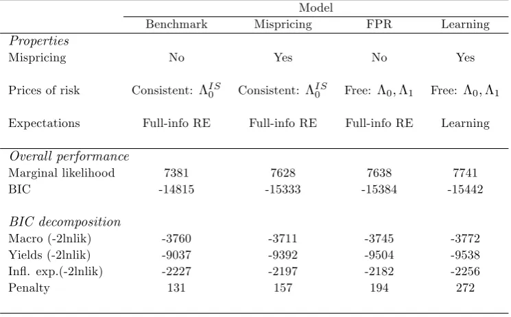
We assess four versions of the macro-…nance model: (i) theBenchmark Model, which assumes rational
ex-pectations and full-information by private agents, imposes consistency between the pricing kernel and the
IS equation (i.e. implied constant prices of risk), and prices bonds according to no-arbitrage restrictions;
(ii) the Mispricing Model, an extension of the benchmark model allowing for liquidity premia, expressed
as constant mispricing terms relative to the no-arbitrage model; (iii) the Flexible Price of Risk Model,
an extension of the benchmark model allowing for ‡exible prices of risk; and (iv) the Learning Model,
a general model including learning by private agents with respect to the long-run in‡ation expectation
and the equilibrium real rate, and also allowing for liquidity premia and ‡exible prices of risk. Table 1
summarizes the di¤erences across the models. Below we specify the parameter vector to be estimated for
each of the versions of the model.
Insert Table1
Benchmark Model (B). The parameter vector for the Benchmark Model is:
B = ; ; h; ; ; y; i; ' ; 'y; 'i; ; y; i; ; ; 0; 0;
y;1; y;2; y;4; y;12; y;20; y;40; ;4; ;40
i0
;
where the parameters 0and 0 are the estimated initial values for the latent variables t and t:
Mispricing Model (Misp). The …rst extension to the benchmark model allows for mispricing in terms
of constant maturity-speci…c deviations of the actual yield curve from the one implied by no-arbitrage
restrictions. Since the mispricing terms, ;are not systematically related to macroeconomic variables,
we refer to them as liquidity e¤ects. We include a liquidity e¤ect for yields with maturities of 2,4, 12,
20and40quarters. The parameter vector in this case is given by:
M isp= 0B; 2; 4; 12; 20; 40
0
:
Flexible Price of Risk Model (FPR). In the benchmark model, the prices of risk are implied by the
structural macroeconomic framework and are time invariant. This version of the model relaxes this
constraint.12 Nevertheless, to reduce the number of parameters to be estimated, we impose some structure
on the prices of risk. We assume that (i) the prices of risk only load on observable macroeconomic
1 1The Metropolis-Hastings algorithm is based on a total of 200,000 simulations with a training sample of 20,000. An
acceptance ratio of 40% is targeted in the algorithm. Parameters are drawn based on the Gaussian random walk model. Finally, we use Geweke (1999)’s test for di¤erences in means and cumulative mean plots to assess convergence.
1 2Hördahl, Tristani, and Vestin (2006) and Rudebusch and Wu (2008) also estimate an alternative version of the structural
variables, t; ytandit;13 and (ii) the prices of risk and the risk premia are stationary under the PLM: 0= 2 6 6 6 6 6 6 6 6 4 0; 0;y 0;i 0; 0; 0 0 3 7 7 7 7 7 7 7 7 5
; 1=
2 6 6 6 6 6 6 6 6 4
1; 1; y 1; i 0 0 0 1; 1; i 1; i 0 0
1;y 1;yy 1;yi 0 0 0 1;y 1;yi 1;yi 0 0
1;i 1;iy 1;ii 0 0 0 1;i 1;ii 1;ii 0 0
1; 1; y 1; i 0 0 0 1; 1; i 1; i 0 0
1; 1; y 1; i 0 0 0 1; 1; i 1; i 0 0
0 0 0 0 0 0 0 0 0 0
0 0 0 0 0 0 0 0 0 0
3 7 7 7 7 7 7 7 7 5 :
Therefore, the parameter vector to be estimated is:
F P R= 0B; 0; ; 0;y; 0;i; 0; ; 0; ; 1; ; 1; y; 1; i; 1;y ; 1;yy; 1;yi; 1;i ; 1;iy; 1;ii
0
:
Learning Model (Learning). The last version of the model includes learning by private agents and allows
for the two extensions of the benchmark model discussed above, i.e. mispricing and ‡exible prices of risk.
As a result, the parameter vector is:
Learning= [ 0F P R; 2; 4; 12; 20; 40; ! ; ! ; g ; g ; b; b; 0b; 0b]0;
where the last eight parameters refer to the learning dynamics explained in Section 2.1.1.
4
Empirical analysis
We describe the data in Section 4.1 and the prior distribution for the parameters in each model version
in Section 4.2. In Section 4.3, we compare the performance of the models by means of the marginal
likelihood and BIC statistics. Since the Learning Model outperforms the other versions of the
macro-…nance model, we discuss the posterior density and implied factors of this model in Sections 4.4 and 4.5,
and the implications for the yield curve in Sections 4.6 and 4.7.
4.1
Data
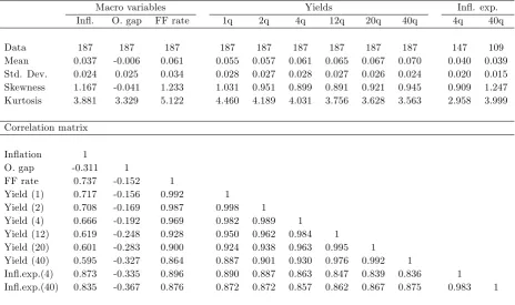
The data set consists of quarterly observations for the U.S. economy covering the period from 1960:Q2
to 2006:Q4 (187 observations). The data include observations on macroeconomic variables, the term
structure of interest rates, and in‡ation expectations. The macroeconomic variables are the in‡ation
rate, the output gap, and the central bank policy interest rate. In‡ation is computed based on the
quarterly GDP de‡ator and is expressed in per annum terms. The output gap is the percentage deviation
of GDP from the potential output reported by the Congressional Budget O¢ce (CBO). The policy rate is
the e¤ective federal funds rate.14 The term structure of interest rate data consist of yields of bonds with
maturities of 1, 2, 4, 12, 20 and 40 quarters. For 1- and 2-quarter yields, we use data from the secondary
market for Treasury bills.15 For 4-, 12-, 20- and 40-quarter yields, we combine the data sets compiled
1 3This type of restriction is based on the statistical tests rejecting the unit root hypothesis for term and risk premia.
In our context, it implies the stationarity of the prices of risk. In the empirical implementation, we restrict 1 further.
Statistical analysis also shows that we can set 1; : and 1; : to zero.
1 4For in‡ation and real GDP, the data series GDPDEF and GDPC1 are retrieved from the Federal Reserve Economic
Data (FRED) data base, respectively. We use the 2006 vintage of potential output. Data on the e¤ective federal funds rate are obtained from the Federal Reserve Bank of St. Louis FRED database.
by Gürkaynak, Sack, and Wright (2007) and McCulloch and Kwon (1993).16 In‡ation expectation data
are obtained from the Survey of Professional Forecasters (SPF) provided by the Federal Reserve Bank of
Philadelphia. We use the series for the 4- and 40-quarter average in‡ation expectation.17
4.2
Priors
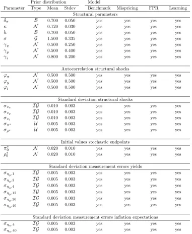
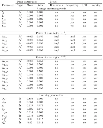
Tables 2 and 3 report the prior distribution, mean, and standard deviation of the parameters of the
respective models. Table 2 lists the priors for the parameters which are common to all models, i.e.
the structural parameters and parameters related to structural shocks and measurement errors. Table 3
contains the priors for the set of parameters which vary according to each model, i.e. related to mispricing,
prices of risk, and learning.
Insert Tables 2 and 3
Phillips curve. We adopt a beta distribution for the in‡ation indexation parameter ( ) with a mean of
0:7and standard deviation of0:05. This attributes a signi…cant role to the endogenous backward-looking
component in in‡ation ( 2; = 0:41). We assume a strict prior for the output sensitivity of in‡ation ( ),
represented by a normal distribution with a mean of0:12and standard deviation of0:03.18
IS curve. For the level of relative risk aversion ( ); we follow the standard macroeconomic view and
adopt a prior with mass concentrated on the lower values of :For this, we choose a gamma distribution
with a mean of 1:5 and standard deviation of0:4.19
Monetary policy. The priors for the monetary policy rule are obtained from the Taylor rule literature.
The in‡ation gap and output gap parameters ( , y) have normal distributions with a mean of0:5. The
di¤erences in the standard deviations (i.e. = 0:25 and y = 0:4) re‡ect the reported uncertainty
in the estimates for these parameters. For the interest rate smoothing parameter ( i), we use a normal
distribution with a mean of0:8 and standard deviation of 0:2. The high standard deviation re‡ects the
ongoing debate concerning the degree of interest smoothing (see Rudebusch (2002), English, Nelson, and
Sack (2003), and Gerlach-Kristen (2004)).
Structural shocks. We use loose priors for the autocorrelation parameters of the three structural shocks,
i.e. a normal distribution with mean and standard deviation equal to 0.5. The standard deviation for the
permanent shocks ( and ) are uniformly distributed with support between 0 and 1% per quarter.
They prevent permanent shocks from becoming excessively large but are su¢ciently wide to include a
signi…cant range for these parameters.
Measurement errors. We use a inverted gamma distribution with a mean of0:005and standard deviation
of0:003for the standard deviation of the measurement errors of bond yields and in‡ation expectations.20 1 6The Gürkaynak, Sack, and Wright (2007) data set starts on the 14th of June 1961 for bonds with maturities of 4,
12 and 20 quarters and on the 16th of August 1971 for the 40-quarter bond. Missing observations are obtained from the McCulloch and Kwon (1993) data set.
1 7Table B1 in the Appendix reports the descriptive statistics of the data.
1 8The value for the mean corresponds to the one found by Bekaert, Cho, and Moreno (2010). This bias towards lower
estimates is in line with estimation results using General Method of Moments (GMM) or Maximum Likelihood (ML) techniques (e.g. Cho and Moreno (2006)).
Mispricing. For the liquidity premia ( ), we use a normal distribution with a mean of 0 and standard
deviation of0:005. This re‡ects a belief on relatively small average mispricing errors.
Prices of risk. We choose relatively uninformative priors for the prices of risk. The priors are set such
that at the mean the model implies (i) a positive constant risk premium (E( 0)< 0); and (ii) a risk
premium increasing with the in‡ation and the interest rate gaps, ( t t) and (it t t); while
decreasing with the output gap, yt:
Learning. We impose relatively strict priors for the parametersw andw :We adopt beta distributions
with support on the interval[0; 1]with a mean of0:85and standard deviation of0:10. The prior is thus
biased towards the full-information RE model.21 For the constant gains (g , g ), we apply a uniform
distribution on the interval[0; 0:25]:This support is su¢ciently large to contain most of the estimates
reported in the literature (e.g. Kozicki and Tinsley (2005a) and Milani (2007)).
4.3
Relative performance of the models
The marginal likelihood of the data and the BIC statistics for each model are reported in Table 1.
The BIC serves as a goodness-of-…t measure up to a penalty for model dimensionality. We assess the
empirical relevance of allowing for mispricing in the macro-…nance model by comparing the performance
of the Benchmark Model with that of the Mispricing Model. We observe that the marginal likelihood
of the Mispricing Model (7628) is signi…cantly higher than the one implied by the Benchmark Model
(7381). This shows the importance of allowing for mispricing terms in the modeling of the yield curve.
Section (4.6) below analyses the estimated mispricing parameters for theLearning Model together with
the analysis of the implied …t of the yield curve.
We now evaluate the e¤ect of time-varying prices of risk on the performance of the macro-…nance
model. Since the marginal likelihood of the Flexible Price of Risk model (7638) is signi…cantly higher
than that of the Benchmark Model (7381), we can reject the implied constant prices of risk which
guarantee consistency between the macroeconomic framework and the pricing kernel ( 0= IS0 , 1= 0).
Nevertheless, in order to assess whether our results also imply a rejection of the extended expectations
hypothesis, which simply postulates time-invariant prices of risk ( 06= 0, 1= 0), we need to determine if the parameters in 1 are statistically di¤erent from zero. This is indeed the case as can be seen in
Table C4 in the Appendix. The results then point to the need to allow for time-varying prices of risk
and, therefore, risk premia in the modeling of bond yields.
The above results indicate that one should incorporate both extensions (mispricing and time-varying
prices of risk) in a macro-…nance model. This is done in theLearning Model. The results show that this
version outperforms all other versions with a marginal likelihood (7741) substantially higher than that for
the alternative models. Therefore, the three extensions combined signi…cantly improve the overall …t of
the model. Assuming a uniform prior over the alternative model versions, the posterior odds ratio of the
learning version equals its Bayes factor of (approximately) 1, suggesting the superiority of this version
2 1This is especially justi…ed for the output-neutral real rate since the data set does not contain much information
relative to all other versions of the model. Results for the BIC statistics in Table 1 lead to a similar
conclusion. Despite the fact that theLearning Model is the largest model, it is clearly preferred in terms
of the BIC statistic.
Table 1 also decomposes the performance of the models in terms of the macroeconomic, yield curve
and in‡ation expectations dimensions. We use the likelihood of the prediction errors of the respective data
subsets as performance measure. This decomposition also shows that the Learning Model outperforms
all other model versions in each dimension. In the sections below, therefore, we only assess the posterior
distribution of the parameters in theLearning Model and its implications for the yield curve.
4.4
Posterior distribution of the
Learning Model
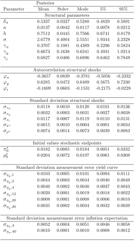
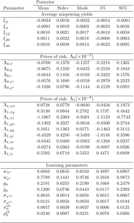
Tables 4 and 5 report the mean, standard deviation, mode, and90%con…dence interval for the posterior
distribution of the parameters in the Learning Model.22 We focus on four sets of parameters related to:
(i) the New-Keynesian macro model; (ii) the structural and belief shocks; (iii) the prices of risk; and
(iv) the learning dynamics. The mispricing parameters are discussed in Section (4.6) where we examine
the implied …t of the yield curve. When not stated di¤erently, the estimates refer to the mode of the
posterior distribution.
Insert Tables 4 and 5
Structural model. The estimates for the structural model in Eqs. (1), (5), and (8) shown in Table 4 are in line with …ndings in the macro literature. The results reject the purely forward-looking New-Keynesian
model in favor of a hybrid version containing also a backward-looking component. The following remarks
can be made with respect to each structural equation.
Phillips curve. The in‡ation indexation parameter ( ) with a mode of0:53 implies a relatively high
weight on the forward-looking in‡ation component, i.e. 1; = 0:66. Such value is typically not recovered
in the macro-…nance literature. For instance, Bekaert, Cho, and Moreno (2010) report implied values in
the range of[0:53;0:63]:Nevertheless, our estimate is aligned with results reported in the macro literature
(e.g. Galí and Gertler (1999) and Galí, Gertler, and David Lopez-Salido (2005)). The estimate for the
mode of the in‡ation sensitivity to the output gap ( ) is relatively small (0:012), despite the strict prior
around a mean value of 0:12: This indicates a weak link between detrended output and in‡ation and
re‡ects the mismatch in the persistence of the two variables. Although lower than theoretically expected,
this estimate is high compared to other General Method of Moments (GMM) or Maximum Likelihood
(ML) based studies (e.g. Cho and Moreno (2006) report a value of 0.001).
IS curve. The habit persistence parameter (h) is estimated at a mode of0:76and with a relatively high
precision:The estimate for the risk aversion parameter ( ) also seems reasonable from a macroeconomic
perspective. Its mode is equal to 2:55 with 90% of the support contained in the interval [1:9; 3:2].23
2 2Appendix C presents the posterior distribution of the parameters for the other versions of the model.
2 3This range of values is quite di¤erent from the ones found in the macro-…nance literature. Dewachter and Lyrio (2008),
Combined, these values result in a relatively strong forward-looking component with a weight on the
expected future output gap ( y) equal to 0:69.
Monetary policy. Our estimates imply an active monetary policy rule both in the in‡ation and output
gaps. Both and y (with modes at0:44and 0:63;respectively) are positive, statistically signi…cant,
and close to the values implied by the standard Taylor rule. We also …nd a relatively low value for
the interest rate smoothing parameter ( i) with a mode of 0:69 in the con…dence interval [0:64; 0:78].
This implies that it would take the FED less than two quarters to halve the gap between the actual
and the target interest rate. We believe this estimate is more realistic than the ones commonly reported
in the literature (around 0:9 on a quarterly frequency) which suggest a halving time of more than six
quarters. Our results are in line with the macro literature, e.g. Trehan and Wu (2007), and underscore
the importance of omitted variable bias in Taylor rule estimations.24
Structural and belief shocks. We estimate the standard deviation of seven shocks in the Learning
Model: three temporary structural macroeconomic shocks, i.e. supply, demand and policy rate shocks
( v , vy, vi); two permanent shocks associated with the in‡ation target and the output-neutral real
rate ( , ); and two belief shocks related to the in‡ation target and the output-neutral real rate
( b, b).
The estimates in Table 4 indicate that the supply and policy rate shocks are relatively large ( v =
0:012 and vi = 0:012) and negatively autocorrelated (' = 0:38 and 'i = 0:15). Although the
negative autocorrelation might be surprising, note that the model incorporates two additional channels
modeling persistence: (i) the endogenous persistence due to in‡ation indexation ( ) and interest rate
smoothing ( i); and (ii) the dependence of in‡ation and the interest rate on the processes modeling the
perceived stochastic endpoints for in‡ation and the output-neutral real rate. Finally, a low …rst-order
correlation for supply and policy rate shocks has also been reported by Ireland (2007). The demand
shock, on the other side, is relatively small ( vy = 0:003) and with a autocorrelation ('y) of0:65.
An important feature of the learning dynamics described in Eq. (13) is the introduction of exogenous
belief shocks. We …nd that, for in‡ation, belief shocks (see Table 5) are relatively large in comparison
with actual in‡ation target shocks ( b = 0:58% compared to = 0:04%). This implies a relatively
smooth in‡ation target dynamics while still allowing for substantial variation in the perceived long-run
in‡ation expectation. On the contrary, shocks to the output-neutral real rate are larger than belief
shocks to this rate ( = 0:73%compared to b = 0:50%). Although this highlights the importance of
output-neutral real rate shocks for the the yield curve dynamics, especially for long-term yields, it could
also point to some form of misspeci…cation of our model. This source of variation is typically ignored in
standard macro-…nance models by assuming a constant equilibrium real rate. Both …ndings are important
departures from the results of standard macro-…nance models.
2 4The omitted variable bias argument in the interest rate smoothing parameter has been put forward by Rudebusch
Prices of risk. As mentioned before, it has been argued by Kozicki and Tinsley (2005b) that models containing asymmetric information and learning dynamics can explain the rejection of the expectations
hypothesis. These authors take into consideration the fact that private agents’ perception about the
central bank’s in‡ation target might deviate from the central bank’s true target. This is relevant since
long-horizon yields are related to long-horizon expectations of the policy rate which includes in‡ation
expectations and the latter are anchored by market perceptions of the central bank’s in‡ation target.
The authors conclude that the common rejection of the expectations hypothesis might re‡ect incorrect
assumptions about expectations formation process and not an incorrect link between long and short
rates. Our estimation results of the Learning Model suggest this is not the case. This can be seen by
the fact that even allowing for learning some of the time-varying prices of risk parameters in 1 remain
signi…cant (see Table 5). In order to reproduce the data dynamics, therefore, it seems crucial to allow for
time-varying risk premia in the dynamics of bond yields.
Learning dynamics. The size and signi…cance of the learning parameters in Table 5 indicate substan-tial deviations from the full-information RE model. Noting that the latter model is embedded in the
Learning Model, i.e. for! =! = 1, it is clearly rejected in favor of the alternative of learning, i.e
0 < ! < 1; 0 < ! < 1. The deviation from the full-information case is especially pronounced for
the perceived long-run in‡ation expectation suggesting that this expectation is weakly anchored. The
signi…cant learning e¤ect is due to (i) a relatively large weight attached to private signals in the updating
rule for the perceived stochastic endpoint for in‡ation (1 ! = 0:35), (ii) a relatively large size of
belief shock ( b= 0:58%), and (iii) a signi…cant constant gain (g = 0:22):As can be seen in Eq. (13),
multiplying the constant gain (g ) by(1 ! )yields the total impact of the subjective forecast error on
the perceived long-run in‡ation rate, which in our case is equal to0:07and in line with estimates reported
in the literature. For instance, Milani (2007) …nds values in the range 0:02 0:03, while Kozicki and
Tinsley (2005a) …nd higher values (around 0:10) using a similar learning model. For the output-neutral
real rate, the estimates imply only marginal e¤ects of learning on its dynamics due to the low weight
given to private signals in the updating rule for the perceived equilibrium real rate (1 ! = 0:03).
4.5
Macro factors implied by the
Learning Model
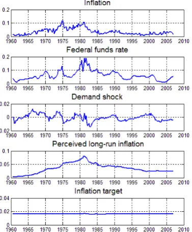
Figure 1 displays the …ltered time series for the ten macroeconomic factors implied by the mode of the
posterior distribution of theLearning Model. They include three observable factors (in‡ation, the output
gap and the federal funds rate), three exogenous shocks (supply, demand and policy rate shocks), and
four stochastic endpoints (actual and perceived) for in‡ation and the output-neutral real rate. Figure2
depicts the actual and perceived stochastic endpoints and the respective 90% con…dence intervals together
with the respective observed macroeconomic variables.
Insert Figure1and2
From Figure 1; we observe the mentioned disconnection between the in‡ation target of the central
signi…cant and persistent di¤erences between the two series. The series for the perceived long-run in‡ation
expectation displays substantial time variation, while the time path of the in‡ation target is mostly
contained within the con…dence interval between1% 3:8%(see top-right panel of Figure2). A similar
type of disconnection between subjective in‡ation expectations and the in‡ation target is found in Kozicki
and Tinsley (2005a) and Dewachter and Lyrio (2008). The results suggest that subjective in‡ation
expectations were not well anchored, especially over the …rst part of the sample.
For the output-neutral real rate, we notice a strong similarity between the actual and perceived rates.
As mentioned before, this is implied by the estimate forw (0:97) in Eq. (13) which assigns a marginal
role to the learning dynamics. Figure 2 shows that the …ltered output-neutral real rate is typically
contained in the interval between0% 5%p.a. (with a historical average close to2:5%p.a.) and displays
signi…cant persistence with relatively low rates in the 1970s and substantially higher rates in the 1980s.
The perceived output-neutral real rate (bottom-left panel of Figure2) also displays signi…cant volatility
and persistence, features also reported by e.g. Laubach and Williams (2003), Clark and Kozicki (2004)
and Bjørnland, Leitemo, and Maih (2008). Figure 2 also illustrates the substantial di¤erences in the
uncertainty surrounding the estimated time paths of the two series. The perceived real rate (bottom-left
panel) is identi…ed with signi…cant more precision than the actual rate (bottom-right panel) due primarily
to the yield curve dynamics. The dynamics of the actual real rate is only weakly identi…ed by the ALM,
as can be observed from its large con…dence interval. In fact, the90%con…dence interval reported in the
bottom-right panel of Figure 2 does not exclude a constant or very smooth actual output-neutral real
rate.
The variability in the perceived output-neutral real rate and the disconnection between the in‡ation
target of the central bank and the subjective in‡ation expectations of private agents help explain a
signi…cant part of the variation in long-term yields. This is done without having to assign an excessively
large standard deviation for the in‡ation target of the central bank.25 The estimated mode for the
in‡ation target is around two percent while the …ltered in‡ation expectations are in line with survey
data (see Figure 2). For the output-neutral real rate, however, its estimated standard deviation might
be excessively large (see Figure1).
4.6
The …t of the yield curve
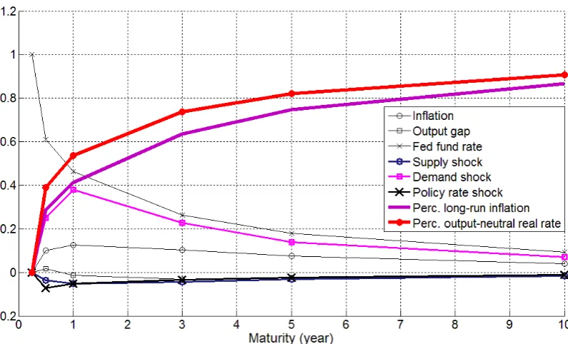
The yield curve model implied by theLearning Model includes eight factors: three observable
macroeco-nomic factors, three exogenous shocks, and two latent factors tracking the perceived stochastic endpoints
for in‡ation and the output-neutral real interest rate.26 Figure3 shows the yield curve loadings, i.e. the
sensitivity of the yield curve with respect to each macroeconomic factor. As can be seen, long-term yields
are a¤ected almost one-to-one by both stochastic endpoints. The factor loadings on the policy rate reveal
a slope factor response, while other macroeconomic variables, i.e. in‡ation and demand shocks, a¤ect
2 5For instance, Doh (2006) reports standard deviations between30and35basis points per quarter for U.S. data for the
period 1960-2005. Dewachter and Lyrio (2006) and Bekaert, Cho, and Moreno (2010) …nd values ranging from30to more than73basis points per quarter.
2 6TheLearning Model features a total of ten factors. However, only the factors entering the PLM are relevant for the
primarily the intermediate maturities.
Insert Figure3
The performance of the model in …tting the yield curve can be assessed by the standard deviation
of the measurement errors ( y; ) in Table 4. For yields with maturity above 2 quarters, this value is
below 40 basis points.27 These values are small relative to the total variation of the yields, which exceed
240 basis points (see Table B1 in the Appendix). These values are also in line with estimates reported
in the macro-…nance literature. For instance, Bekaert, Cho, and Moreno (2010) report measurement
error standard deviations of 45 and 54 basis points for the 4- and 40-quarter yields. Estimates based on
comparable models presented in Dewachter and Lyrio (2008) are around 50 basis points. Interestingly,
De Graeve, Emiris, and Wouters (2009) report signi…cantly lower measurement errors (of the order of
10 to 20 basis points). Comparing these statistics, we conclude that the Learning Model is relatively
successful in explaining the yield curve variation in terms of macroeconomic shocks. More than 95% of
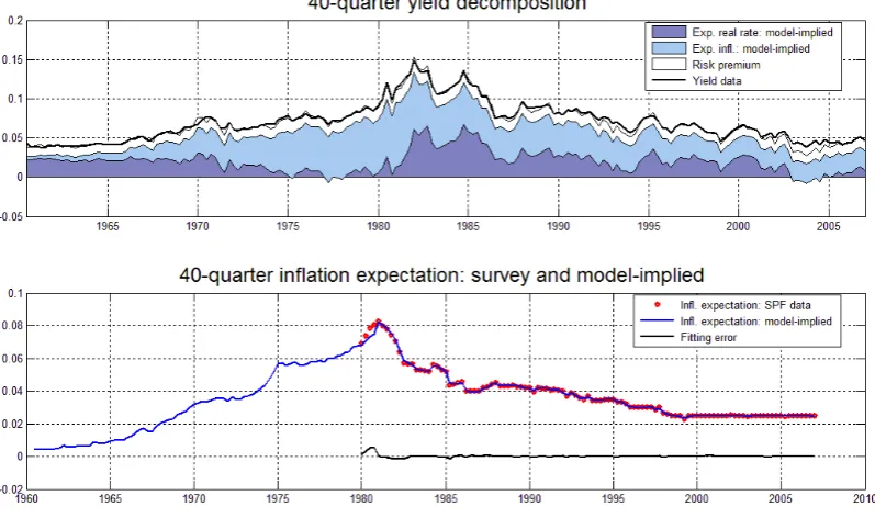
the unconditional variance in yields with maturities beyond 4 quarters is explained by the model. Figure
4 illustrates the yield curve …t implied by the model and Figure 5 decomposes the …t of the 40-quarter
yield into a expected real rate, expected in‡ation and risk premium component. The top panel in this
…gure shows the signi…cant contribution of the expected in‡ation in the composition of the 40-quarter
yield. The bottom panel shows the …t of the model-implied in‡ation expectation with respect to the one
provided by the Survey of Professional Forecasters.
Insert Figures4and5
Despite the large number of factors included in the model, the average mispricing ( ) seems
econom-ically important and increasing with maturity up to 20 quarters (see Table 5), i.e. model-implied yields
are too high at the short end (negative liquidity premium) and too low at the long end of the yield curve
(positive liquidity premium).28 Nevertheless, only the negative mispricing term at the short end of the
yield curve ( 2) is statistically signi…cant.
Finally, Figure 6 displays the expected excess holding return (per annum for a quarterly holding
period) expressed in Eq. (22) together with the NBER recession dates.29 As can be observed, risk
premia have an important time-varying component ranging from 2% p.a. in 1965 to more than 6%
p.a. in 1984 for the 40-quarter maturity bond. Similar time patterns and orders of magnitude have
been reported by Du¤ee (2002) and Campbell, Sunderam, and Viceira (2009). In line with intuition, the
observed risk premia are countercyclical, generating large and positive risk premia during recessions and
2 7A remarkable aspect of the data is the bad …t of the short end of the yield curve with …tting errors around one percent.
This …nding is due to the choice of policy rate. With the federal funds rate representing the policy rate, there is an obvious tension with short-term Treasury rates, given that on average these have been below the federal funds rate. This persistent gap is picked up in the measurement error.
2 8The negative liquidity premium at the short end of the yield curve should not come as a surprise. The positive spread
between the federal funds rate and the short-term treasuries is well documented and is typically attributed to a risk premium in the federal funds rate re‡ecting private banks’ uncertainty over reserve management.
2 9The average excess holding return and standard deviation (in brackets) implied by the data are: 1:1%(0:2%), 1:5%
smaller and even negative risk premia during expansions.30
Insert Figure6
4.7
What factors drive the yield curve?
We turn to the identi…cation of the macroeconomic factors driving monetary policy and the yield curve.
Monetary policy is identi…ed by the federal funds rate and the yield curve is decomposed into its level,
slope and curvature factors. We follow the literature (e.g. Bekaert, Cho, and Moreno (2010)) by
identify-ing (i) the level factor as the average yield across maturity, (ii) the slope factor as the 40-quarter maturity
yield spread (relative to the 1-quarter yield), and (iii) the curvature factor as the sum of the 40-quarter
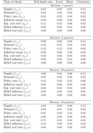
and 1-quarter yields minus two times the 4-quarter yield. Table 6 presents the variance decomposition for
the federal funds rate and the level, slope and curvature factors for horizons of 1, 4, 20 and 40 quarters.
The results show that the high frequency variation in the monetary policy is largely due to independent
monetary policy shocks. Such shocks account for over80%of the 1-quarter variation in the federal funds
rate, with macroeconomic shocks having only a marginal contribution.31 Supply and demand shocks
become more important for intermediate horizons, which is explained by the presence of interest rate
smoothing. At the 4-quarter horizon, supply and demand shocks account for25%of the total variation in
the policy rate. For longer horizons, monetary policy is dominated by long-term equilibrium forces. For
a 40-quarter horizon, movements in the federal funds rate are mostly due to movements in the
output-neutral real rate (75%), with belief shocks to long-run in‡ation expectations accounting for another10%.
Insert Table 6
The variance decomposition of the level factor contradicts the results of standard macro-…nance
models, which attribute most of its variation to long-run in‡ation expectations, e.g. Doh (2006) and
De Graeve, Emiris, and Wouters (2009). Our results indicate that, for all horizons, shocks to the
output-neutral real rate are responsible for most of the variation in the level factor, explaining 85% of the
variation for the 40-quarter horizon. Policy rate shocks are also signi…cant for short-term horizons (up
to 4 quarters) with a smaller contribution of supply shocks. Finally, belief shocks to long-run in‡ation
expectations become relevant for intermediate and long horizons.
The variance decomposition for the slope and curvature factors are more in line with standard
macro-…nance models (e.g. Bekaert, Cho, and Moreno (2010)). The variation in both factors and for all horizons
is dominated by exogenous monetary policy shocks. For the slope factor, demand shocks have a signi…cant
impact for horizons of 4 quarters and above, while for the curvature factor this impact is present for all
horizons.
3 0Rudebusch, Sack, and Swanson (2007) show that a decline in the term premium has been associated with a stimulus
to the economy.
5
Conclusion
We estimate a New-Keynesian macro-…nance model of the yield curve incorporating learning by private
agents with respect to the long-run expectation of in‡ation and the equilibrium real interest rate. Private
agent’s perception about these two variables are updated taking into consideration their own belief shocks
and a constant gain learning process. A preliminary analysis shows that some liquidity premia, expressed
as some degree of mispricing relative to no-arbitrage restrictions, and time variation in the prices of risk
are important features of the data. These features are, therefore, included in our Learning Model.
The Learning Model succeeds to some extent in explaining the yield curve movements in terms of
macroeconomic shocks. Interestingly, the variability in the perceived stochastic endpoints for in‡ation
and the equilibrium real rate turn out to be important in explaining the variability of long-term yields.
The results for this model also show an important di¤erence between the estimated in‡ation target of
the central bank and the perceived long-run in‡ation expectation of private agents. This is especially the
case for the period from the mid-1970s to the mid-1990s and show that private agents’ perceptions about
long-term in‡ation were weakly anchored.
The structural decomposition of the yield curve into its macroeconomic components also provides
new insights concerning the interpretation of the level, slope and curvature factors. For the slope and
curvature factors, the decomposition generated by the Learning Model is in line with standard
macro-…nance models. These factors are primarily a¤ected by exogenous monetary policy shocks, with demand
shocks contributing substantially. For the level factor, standard models attribute most of its variation
to long-run in‡ation expectations. We …nd, however, that shocks to the output-neutral real rate are
responsible for most of the variation in this factor. We should emphasize that the pronounced variability
of the output-neutral real rate could be a sign of model misspeci…cation.
Several extensions of the model could be undertaken. First, our results document the signi…cance
of mispricing terms within a structural macro-…nance model. This mispricing can be quite substantial,
especially at the short end of the yield curve, suggesting the need for further analysis of these results. In
recent research, Dewachter and Iania (2010) show the importance of including …nancial factors related
to the overall liquidity and counterparty risk in the money market in the modeling of the yield curve.
The inclusion of such factors in our framework could eliminate the signi…cance of such mispricing terms.
Second, in this paper, we use a short-cut to identify the output-neutral real rate. Given the importance
of this factor for long-term yields, an important task is to verify further the interpretation of this factor
within a learning model. To this end, our model could be extended with the introduction of a complete
micro-founded supply side. Such an extension would facilitate the identi…cation of the long-run real
interest rate and would re…ne the set of observable macroeconomic shocks, as in De Graeve, Emiris, and
References
Ang, A.,andM. Piazzesi(2003): “A No-Arbitrage Vector Autoregression of Term Structure Dynamics
with Macroeconomic and Latent Variables,”Journal of Monetary Economics, 50(4), 745–787.
Bekaert, G., S. Cho, and A. Moreno (2010): “New-Keynesian Macroeconomics and the Term
Structure,”Journal of Money, Credit and Banking, 42, 33–62.
Bjørnland, H. C., K. Leitemo, and J. Maih (2008): “Estimating the Natural Rates in a Simple
New Keynesian Framework,” Working Paper 2007/10, Norges Bank.
Calvo, G. A. (1983): “Staggered Prices in a Utility-Maximizing Framework,” Journal of Monetary
Economics, 12(3), 383–398.
Campbell, J. Y., A. Sunderam, and L. M. Viceira (2009): “In‡ation Bets or De‡ation Hedges?
The Changing Risks of Nominal Bonds,” NBER Working Papers 14701, National Bureau of Economic
Research, Inc.
Cho, S.,andA. Moreno(2006): “A Small-Sample Study of the New-Keynesian Macro Model,”Journal
of Money, Credit and Banking, 38(6), 1461–1481.
Chun, A. L. (2011): “Expectations, Bond Yields, and Monetary Policy,”Review of Financial Studies,
24(4), 208–247.
Clark, T. E., and S. Kozicki (2004): “Estimating Equilibrium Real Interest Rates in Real-Time,”
Discussion Paper Series 1: Economic Studies 2004,32, Deutsche Bundesbank, Research Centre.
De Graeve, F., M. Emiris, and R. Wouters(2009): “A Structural Decomposition of the US Yield
Curve,”Journal of Monetary Economics, 56(4), 545–559.
Dewachter, H., and L. Iania(2010): “An Extended Macro-Finance Model with Financial Factors,”
Journal of Financial and Quantitative Analysis, forthcoming.
Dewachter, H., and M. Lyrio (2006): “Macro Factors and the Term Structure of Interest Rates,”
Journal of Money, Credit and Banking, 38(1), 119–140.
(2008): Learning, Macroeconomic Dynamics, and the Term Structure of Interest Rates, Asset
prices and monetary policy. NBER.
Doh, T. (2006): “Estimating a Structural Macro Finance Model of the Term Structure,” Discussion
paper.
(2007): “What Does the Yield Curve Tell Us about the Federal Reserve’s Implicit In‡ation
Target?,” Research Working Paper RWP 07-10, Federal Reserve Bank of Kansas City.
Duffee, G. R. (2002): “Term Premia and Interest Rate Forecasts in A¢ne Models,” The Journal of