Resolution of Resource Contentions in the CCPM MPL Using Simulated Annealing and Genetic Algorithm

http://www.scirp.org/journal/ajor ISSN Online: 2160-8849

ISSN Print: 2160-8830

Resolution of Resource Contentions in the

CCPM-MPL Using Simulated Annealing

and Genetic Algorithm

Hajime Yokoyama, Hiroyuki Goto

Department of Industrial & System Engineering, Hosei University, Tokyo, Japan

Abstract

This research aims to plan a “good-enough” schedule with leveling of resource con-tentions. We use the existing critical chain project management-max-plus linear framework. Critical chain project management is known as a technique used to both shorten the makespan and observe the due date under limited resources; the max- plus linear representation is an approach for modeling discrete event systems as production systems and project scheduling. If a contention arises within a single re-source, we must resolve it by appending precedence relations. Thus, the resolution framework is reduced to a combinatorial optimization. If we aim to obtain the exact optimal solution, the maximum computation time is longer than 10 hours for 20 jobs. We thus experiment with Simulated Annealing (SA) and Genetic Algorithm (GA) to obtain an approximate solution within a practical time. Comparing the two methods, the former was beneficial in computation time, whereas the latter was bet-ter in bet-terms of the performance of the solution. If the number of tasks is 50, the solu-tion using SA is better than that using GA.

Keywords

Critical Chain Project Management, Max-Plus Algebra, CCPM-MPL, Simulated Annealing, Genetic Algorithm

1. Introduction

This research aims to plan a “good-enough” schedule with leveling of resource conten-tions. References [1] and [2] modified and extended a scheduling methodology referred to as critical chain project management-max-plus linear (CCPM-MPL), in which CCPM [3][4] was applied to the max-plus algebra [5]. CCPM is a technique for project

How to cite this paper: Yokoyama, H. and Goto, H. (2016) Resolution of Resource Contentions in the CCPM-MPL Using Si-mulated Annealing and Genetic Algorithm. American Journal of Operations Research, 6, 480-488.

http://dx.doi.org/10.4236/ajor.2016.66044

Received: September 20, 2016 Accepted: November 18, 2016 Published: November 21, 2016

Copyright © 2016 by authors and Scientific Research Publishing Inc. This work is licensed under the Creative Commons Attribution International License (CC BY 4.0).

http://creativecommons.org/licenses/by/4.0/

management invented by E. M. Goldratt and developed by L. P. Leach. The objective of this method is to both shorten the makespan and observe the due date under a limited number of resources. The max-plus algebra is an algebraic system wherein the max and plus operations are defined as addition and multiplication, respectively. MPL [1] repre-sentation is an approach for modeling and analyzing a class of discrete-event systems such as production and project scheduling, in which the behavior of the target system is represented by linear equations in the max-plus algebra. MPL representation can for-mulate systems with structures of non-concurrency, synchronization, parallel pro- cessing of multiple tasks, and so on [1]. We assume that a single resource cannot process multiple tasks simultaneously. If a contention arises within a single resource, we must resolve it by appending precedence relations. Thus, the resolution framework is reduced to a combinatorial problem. To level resource contentions, we developed a complete enumeration method by which an exact solution is obtained. In a numerical simulation, the maximum computation time was longer than 10 hours for 20 jobs. Ref-erence [6] obtained a “good-enough” schedule by using Genetic Algorithm (GA) within a short computation time. On the other hand, we uncovered a preliminary design to obtain a “good-enough” schedule by using Simulated Annealing (SA) [7]. However, it is not currently clear which of the two methods is better. Hence, this research compares the two methods in terms of the performances of their solutions, computation times, and values.

2. CCPM-MPL Framework

After defining the max-plus algebra, we define the CCPM-MPL framework with the help of [1] and [2].

2.1. Max-Plus Algebra

We define a set



max

=





{ }

−∞

, where  is the whole real line. Then, for max

,

x y∈ , we define the operators:

( )

max

,

,

x

⊕ =

y

x y

(1) .

x⊗ = +y x y (2)

The priority of operator ⊗ is higher than that of ⊕ . If

,

max

m n×

∈

X Y



and

max

n q×

∈

Z



,

[

] [ ] [ ]

, ij ij ij

⊕ = ⊕

X Y X Y (3)

[

]

max 1

[ ] [ ]

.

n k

ij = ik kj

⊗ = ⊗

X Z X Y (4)

The zero and unit elements for operators ⊕ _and ⊗ _{are denoted by}

ε = −∞

(

)

and

e

( )

=

0

, respectively.

ε

is a matrix whose elements are all

ε

, and e is a matrix

whose diagonal elements are e and whose off-diagonal elements are

ε

. If

X

∈



_maxn n× ,

the following operator *

X is the Kleene star:

( )1

* 2

,

s

⊗ − ⊗

= ⊕ ⊕

⊕ ⊕

where

s

(

1

≤ ≤

s

n

)

is an instance that satisfies X⊗ −( )s 1 ≠

ε

and ⊗s ₌

X ε . In

addi-tion, we define

\ .

x y= − +x y (6)

2.2. Formulation of the CCPM-MPL Framework

We define the following relevant matrices and vectors:

• _{n: number of tasks;}

• p: number of external outputs;

• q: number of external inputs;

• ₀

∈

_maxn q×

B



: input matrix,

[ ]

₀

ij

B = {e: if task i has an input transition j, ε:

other-wise};

• ₀

∈

_maxp n×

C



: output matrix,

[ ]

₀

ij

C = {e: if task j has an output transition i, 𝜀𝜀:

other-wise};

• ₀

∈

_maxn n×

F



: adjacency matrix,

[ ]

₀

ij

F = {e: if task i has a preceding task j, ε:

other-wise};

•

∈

_maxn

d



: system parameter,

[ ]

i

d : duration time in task i;

•

_∈

_maxq

u



: input vector,

[ ]

i

u : input time to external input i;

•

_∈

_maxp

y



: output vector,

[ ]

i

y : output time from external output i;

•

_∈

_maxn

x



: state vector,

[ ]

i

x : start or completion time of task i.

The earliest task-completion times of all tasks, xE, are calculated using E= 0⊗ 0⊗ ,

x A B u (7)

where

(

)

* 0 = 0⊗ 0 ⊗ 0,

A P F P

(8)

( )

0

=

diag

.

P

d

(9)

Matrixes A0 and P0 are the transition and weight matrices, respectively. The

ear-liest output times to all output transitions, yE, are then calculated by E= 0⊗ E.

y C x

(10)

Then, the latest task-starting times, xL, are calculated using Equation (10):

(

)

L

=

0

⊗

0

\

E

.

x

C

A

y

(11)

The latest input times, uL, are calculated in terms of xL: L = 0\ L.

u B x (12)

As a consequence, the total floats of all tasks can be calculated using Equations ((5) and (8)):

(

)

0

=

L

+

−

E

.

m

x

d

x

(13)

All tasks can be classified into two types:

[ ]

m0 _i =0 and

[ ]

m0 _i >0 are a critical and

a non-critical task, respectively. We define two vectors, 0

,

0 max

n

∈

a b



, to classify each

[ ]

a0 i=

{

e: if

[ ]

m0 i=0,ε: if

[ ]

m0 i >0 ,

}

(14)

[ ]

b0 i=

{

e: if

[ ]

m0 i>0,ε: if

[ ]

m0 i =0 .

}

(15)

We then calculate two matrices, a

,

b max

n n×

∈

P P



, as follows:

( )

a

=

diag

0

⊗

P

0

,

P

a

(16)

( )

b

=

diag

0

⊗

P

0

.

P

b

(17)

In the CCPM framework, there are two types of buffers, referred to as feeding and project buffers. The size of each buffer is calculated by

(

)

*

feed = b⊗ 0⊗ b ⊗ 0 2 ,

r P F P g (18)

(

)

*

proj = a⊗ 0⊗ a ⊗ 0 2 ,

r P F P g (19)

where

[

]

T

0 max.

n

e e e

= ∈

g  

(20)

Feeding buffers are inserted wherever a non-critical task joins into a critical one. A project buffer is inserted on the eve of an output to avoid tardiness of the project. To reflect the insertion of the two types of buffers, we incur weights to the adjacency ma-trix F0 and the output matrix C0:

( )

( )

bufs

=

0

⊕

diag

0

⊗

0

⊗

diag

feed

,

F

F

a

F

r

(21)

( )

( )

bufs = 0⊗diag proj ⊕diag feed .

C C r r (22)

Now we can calculate the earliest task-completion, xE′, and the output time, yE′,

after inserting the time buffers. The earliest task-completion times of all nodes, xE′, are

calculated using

E 0 0 ,

′ = ′⊗ ⊗

x A B u (23)

(

)

*

0′ = 0⊗ bufs⊗ 0 .

A P F P (24)

Matrix A0′ is the transition matrix, in which the insertion of the two types of buffers

is reflected. The earliest output times to all output transitions, yE′, are then calculated

by

E bufs E.

′ = ⊗ ′

y C x (25)

We treat yE′ as the objective function and consider minimizing

[ ]

yE′ i.

3. Resolution of Resource Contentions

We explain the resolution of resource contentions with the help of [8]. We add relevant matrices and vectors as follows:

• l: number of resources,

• s: maximum number of tasks that a single resource processes, •

_∈

l s×

S



: processing order of tasks,

[ ]

{

: resource processes task in the th processing, 0 : otherwise

}

ij = k i k j

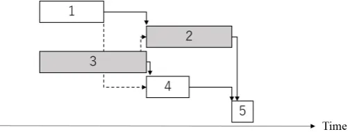
We consider Figure 1 as an example project with five tasks before the leveling of re-source contentions. The duration time of each task is

[

]

T

3 4 5 2 1 =

d . The

adja-cency matrix, F0, is

0 .

e

e

e e

ε ε ε ε ε

ε ε ε ε

ε ε ε ε ε

ε ε

ε ε

ε

ε

ε

 

 

 

 

=

 

 

 

 

F

(26)

Tasks 1, 4, and 5 are processed by resource 1, whereas tasks 2 and 3 are processed by resource 2. If resource 2 processes tasks 2 and 3 simultaneously, a resource contention occurs. We avoid contentions between tasks 2 and 3 by appending two precedence rela-tions, which are expressed by broken arrows in Figure 2, which shows the project after the resource contention is leveled. We then reflect the leveling of the resource conten-tions using the following adjacency matrix, F0′:

0 .

e e

e e

e e

ε ε ε ε ε

ε

ε ε

ε ε ε ε ε

ε

ε ε

ε

ε

ε

 

 

 

′ = 

 

 

 

 

F (27)

In addition, the processing order of tasks, S, is 1 4 5

. 3 2 0

 

=  

 

S (28)

[image:5.595.246.509.453.551.2]

Our numerical simulation to level resource contentions shows that the maximum

Figure 1. Example of a fifth-task project before a resource contention is leveled.

[image:5.595.250.501.588.683.2]

computation time was longer than 10 hours for 20 jobs. We thus consider the develop-ment of approximate methods within a short computation time.

4. Two Metaheuristics

We experiment with an optimization based on Genetic Algorithm (GA) and Simulated Annealing (SA), both of which are common metaheuristics.

4.1. Genetic Algorithm

We experiment with an optimization based on the GA developed in [6], which is used to obtain an approximate solution.

Algorithm 1: Genetic Algorithm

STEP 1. Set mutation parameter and termination condition, mut and i, respectively.

STEP 2. Generate a random solution, S, and create the earliest output times,

[ ]

yE1′ i.

STEP 3. Focusing on a row vector of S that gives the list of tasks for a single

re-source, split the vector into two. We then swap the two vectors, followed by generating a new solution, S′.

STEP 4. If a mutation occurs having probability mut, then proceed to STEP 5.

Other-wise, i.e., if a mutation does not occur, then follow STEP 6. STEP 5. Swap two tasks of S′ at the same resource randomly.

STEP 6. Create the new earliest output times,

[ ]

yE 2′ i using S′.

STEP 7. If

[ ] [ ]

yE 2′ i< yE1′ i follows, then set S:=S′ and

[ ] [ ]

yE1′ i:= yE 2′ i.

STEP 8. Terminate if the termination condition is satisfied. If otherwise, return to STEP4.

4.2. Simulated Annealing

SA [9] is known as an approach to efficiently obtain an approximate solution. We use the 2-opt neighborhood method [10] based on a local search to generate a neighboring solution.

Algorithm 2: Simulated Annealing

STEP 1. Initialize the temperature and cooling parameters, T0 and γ, respectively.

STEP 2. Generate a random solution, S, and create the earliest output times,

[ ]

yE1′ i.

STEP 3. Generate a neighboring solution, S′, and create the new earliest output

times,

[ ]

yE 2′ i.

STEP 4. Calculate ∆ =E

[ ] [ ]

yE 2′ i− yE1′ i.

STEP 5. If ∆ <E 0 holds, then set S:=S′ and

[ ] [ ]

y_E1′ _i:= y_{E 2}′ _i with probably 1.

Otherwise, i.e., if ∆ ≥E 0 _{holds, then set S:=S′ and}

[ ] [ ]

E1′ i:= E 2′ i

y y with

probably

exp

(

− ∆

E T

)

.

STEP 6. Update the temperature parameter, 0

(

0.8 0.99

)

k k

T =

γ

T ≤ ≤

γ

.The value of γ is a cooling parameter which decreases the temperature parameter, T0.

STEP 7. Repeat STEPS3-6.

5. Approximate Ratio and Computation Time

We obtain solutions using the SA- and GA-based algorithms. We use a personal com-puter with the following execution environment:

• _{machine: Dell Optiplex 9020;}

• _{CPU: Intel}® _{Core™ i7-4790 3.60 GHz;}

• _{OS: Microsoft Windows 7 Professional;} • _{memory: 4.0 GB;}

• _{programming language: MATLAB R2015b.}

The test cases for the numerical experiment are generated under the following condi-tions:

• _{number of cases: 100;}

• _{number of resources,} l: for 10, 15, and 20 tasks, we set the number of resources to

3, 5, and 7, respectively;

• _{number of resources for task,} i: uniformly random integer numbers;

• _{duration time,}

[ ]

i

d : uniformly random integer numbers.

We obtain approximate solutions using two metaheuristics. The temperature and cooling parameter are set to T=1 and

γ

=0.85, respectively, for the SA-based

algo-rithm. The mutation parameter and the end condition are set to mut =0.2 and

200

i= , respectively, for the GA-based algorithm. We compare the exact and

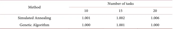
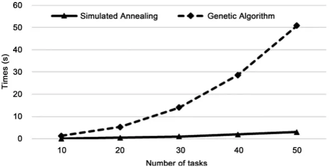
approx-imate solutions. The performance of the solution is shown in Table 1 for the two me-taheuristics. We can confirm that the performance of the solution using the GA-based algorithm is smaller than that using the SA-based algorithm. The average computation times are shown in Figure 3. We can confirm that the computation using the SA-based algorithm is faster than that using the GA-based algorithm. The computation time of the GA-based algorithm is more than16-fold longer than that of the SA-based algo-rithm. The average values of the solutions are shown in Table 2. If the number of tasks is 10 or 20, the values of the solutions using the two methods are not remarkably dif-ferent; if the number of tasks is 30 or 40, the value of the solution using the GA-based algorithm is smaller than that of the SA-based algorithm. However, we should note

Table 1. Performance of the solutions.

Method Number of tasks

10 15 20

Simulated Annealing 1.001 1.002 1.006

[image:7.595.194.554.544.606.2]

Genetic Algorithm 1.000 1.001 1.000

Table 2. Average values of the solutions.

Method Number of tasks

10 20 30 40 50

[image:8.595.210.538.69.236.2]

Figure 3. Average computation times in seconds.

here that the solution using the SA-based algorithm is better than that using the GA if the number of tasks is 50.

6. Conclusions

This research has studied the planning of a “good-enough” schedule with leveling of resource contentions. We utilized an existing framework called the CCPM-MPL. The resolution framework was reduced to a combinatorial problem. We used SA- and GA-based algorithms to obtain approximate solutions within short time. Moreover, we used the 2-opt neighborhood to generate a neighboring solution in the SA-based algo-rithm. Comparing the two methods, the SA-based algorithm was beneficial in terms of computation time, whereas the latter was better in terms of the performance of the so-lution. In addition, when the number of tasks was 50, the value of the solution using the SA-based algorithm was better than that using the GA-based algorithm.

Developing an original heuristic to level resource contentions within a short compu-tation time is our future work.

References

[1] Goto, H. (2017) Forward-Compatible Framework with Critical-Chain Project Management using a Max-Plus Linear Representation. OPSEARCH, 54, 16 p..

http://dx.doi.org/10.1007/s12597-016-0276-3

[2] Goto, H., Truc, N.T.N. and Takahashi, H. (2013) Simple Representation of the Critical Chain Project Management Framework in a Max-Plus Linear Form. SICE Journal of Con-trol, Measurement, and System Integration, 6, 341-344.

http://dx.doi.org/10.9746/jcmsi.6.341

[3] Goldratt, E.M. (1997) Critical Chain. North River Press, Great Barrington.

[4] Leach, L.P. (2005) Critical Chain Project Management. 2nd Edition, Artech House, Boston. [5] Heidergott, B., Olsder, G.J. and Woude, L. (2006) Max Plus at Work: Modeling and

Analy-sis of Synchronized Systems. Princeton University Press, New Jersey.

Japa-nese)

[7] Yokoyama, H. and Goto, H. (2016) Resolution of Resource Contentions in the Critical Chain Project Management Based on Simulated Annealing. Proceedings of the 6th Interna-tional Conference on Industrial Engineering and Operations Management, Kuala Lumpur, 8 March 2016, 29.

[8] Koga, H., Goto, H. and Chiba, E. (2014) Resolution of Resource Conflicts in the CCPM Framework Using a Local Search Method. Proceedings of the IEEE International Confe-rence on Industrial Engineering and Engineering Management, Bandar Sunway, 10 De-cember 2014, 94-98. http://dx.doi.org/10.1109/ieem.2014.7058607

[9] Kirkpatrick, S., Gelatt, C.D. and Vecchi, M.P. (1983) Optimization by Simulated Annealing.

Science, 220, 671-680. http://dx.doi.org/10.1126/science.220.4598.671

[10] Croes, G.A. (1958) A Method for Solving Traveling-Salesman Problems. Operation Re-search, 6, 791-812. http://dx.doi.org/10.1287/opre.6.6.791

Submit or recommend next manuscript to SCIRP and we will provide best service for you:

Accepting pre-submission inquiries through Email, Facebook, LinkedIn, Twitter, etc. A wide selection of journals (inclusive of 9 subjects, more than 200 journals)

Providing 24-hour high-quality service User-friendly online submission system Fair and swift peer-review system

Efficient typesetting and proofreading procedure

Display of the result of downloads and visits, as well as the number of cited articles Maximum dissemination of your research work

Submit your manuscript at: http://papersubmission.scirp.org/