Measuring regional environmental efficiency: A directional distance function approach

Munich Personal RePEc Archive

Measuring regional environmental

efficiency: A directional distance function

approach

Halkos, George and Tzeremes, Nickolaos

University of Thessaly, Department of Economics

2011

Measuring regional environmental efficiency: A

directional distance function approach

By

George E. Halkos

∗

and Nickolaos G. Tzeremes

University of Thessaly, Department of Economics,

Korai 43, 38333, Volos, Greece

Abstract

This paper by applying a directional distance function approach measures the UK regions’ municipality waste performance. In addition the paper constructs conditional stochastic kernels trying to determine nonparametrically the association of regions’ GDP per capita levels with their calculated regional environmental efficiencies. There are evidences of regional environmental inefficiencies for the majority of UK regions regardless their regional GDP per capita levels.

Keywords: Regional environmental performance; Directional distance function; Conditional stochastic kernel

JEL classification: C6, O13, Q5.

∗_{Address for Correspondence:}

1. Introduction

The measurement of environmental technology has been an open challenge for

researchers. The problem lies on the treatment of the pollutant1 in production function

framework. One of the ways that the ‘bad’ output can be modelled appeared in the

pioneered work by Färe et al. (1989) by assuming strong (for desirable outputs) and

weak (for undesirable outputs) disposability treating environmental effects as

undesirable outputs in a hyperbolic efficiency measure. Generally the property of

weak disposability of detrimental variables is well known and has been used in

several formulations (Färe et al., 1996, 2004; Chung et al., 1997; Tyteca, 1996, 1997;

Zofio and Prieto, 2001). But, although this approach is widely accepted among the

environmental economists it has faced several criticisms (Hailu and Veeman, 2001;

Färe and Grosskopf, 2003; Hailu, 2003, Kuosmanen, 2005; Färe and Grosskopf, 2009;

Kuosmanen and Podinovski, 2009).

Our study applies the weak disposability assumption in a directional distance

function measure in order to determine for the first time the environmental

performance of UK regions.

2. Data and Methodology

In our analysis we use data collected we use data collected from two different

regional databases (Eurostat2 and OECD3) and concerning the year 2005. The two

inputs used in our analysis are total regional labour force and regional gross fixed

capital formation (in million Euros). In addition the two outputs used in our study are

regional gross domestic product (million PPS- good output) and as ‘bad’ output

1

The pollutant is also referred to the literature of measuring environmental technology as ‘bad’ output.

2

Available from: http://epp.eurostat.ec.europa.eu/portal/page/portal/region_cities/introduction

3

municipal waste (in 1000t). The data are referring to NUTS 2 level of the UK

regions4.

Therefore, following Färe and Grosskopf (2004) we let P x

( )

to denote an

input vector x∈ℜN₊ which can produce a set of undesirable outputs u∈ℜK₊ and

desirable outputsy∈ℜM₊ . Then in order to determine the environmental technology

several assumptions are needed to be taken following Shephard (1970), Shephard and

Färe (1974) and Färe and Primont (1995). We assume that the output sets are closed

and bounded and that inputs are freely disposal. In addition P x

( )

can be an

environmental output set if:

1.

( )

y u, ∈P x

( )

and 0≤ ≤θ 1 then

(

θ θy, u

)

∈P x

( )

(i.e. the outputs are weakly

disposable) and

2.

( )

y u, ∈P x

( )

, u=0 implies that y=0 (i.e. the null jointness assumption of good

and bad outputs).

The weak disposability assumption implies that the reduction of bad outputs

are costly and therefore the reduction of bad outputs can be obtained only by a

simultaneous reduction of good outputs. In addition the assumption which indicates

that the good outputs are null-joint with bad outputs implies that the bad outputs are

byproducts of the production process when producing good outputs. In order to

formalize the environmental efficiency we use data envelopment analysis (DEA)

framework. Let k=1,...,Kbe the observations and then the environmental output can

be formalized as:

4

For information regarding UK’s regions see:

( ) ( )

}

1

1 1

, : , 1,..., ,

, 1,..., ,

, 1,..., ,

0, 1,...,

K

k km m k

K

k kj j k

K

k kn n k

k

P x y u z y y m M

z u u j J

z x x n N

z k K

= = = ⎧ =_⎨ ≥ = ⎩ = = ≤ = ≥ =

∑

∑

∑

(1) , 1,..., k

z k= K indicate the intensity variables which are not negative and imply

constant return to scale5. The inequality on the good outputs and the equality on the

bad outputs help us to impose the weak disposability assumption and only strong

disposability of good outputs. However the null-jointness is imposed by the following

restrictions on bad outputs:

1 1

0, 1,..., ,

0, 1,..., .

K kj k J kj j

u j J

u k K

=

=

> = > =

∑

∑

(2).

Furthermore, we apply the directional distance function approach as in Chung

et al. (1997) and in order to be able to reduce bad and expand good outputs. In order

to be able to model that in the directional distance function setting we use a direction

vectorg=

(

g_y,−g_u

)

, where g_y =1 and −g_u = −1. Then the efficiency score for a region k'can be obtained from:

(

)

(

)

( )

' ' '

' '

, , ; max

. . ,

k k k o

k k

y u

D x y u g

s t y g u g P x

β

β β

→

=

+ − ∈ (3),

then the linear programming problem can be calculated as:

5

Following Zelenyuk and Zheka (2006, p.149) our regional environmental efficiency measurement follows the most common assumption made in economics which is the constant returns to scale (CRS) assumption. In addition the CRS assumption provides as with greater discriminative power among the examined regions. Finally, due to the fact that we have a small sample size (37 regions) it is therefore better for our analysis to use more robust scale assumptions. However, if the variable returns are

needed to be calculated the

1 1

K k k= z =

(

' ' '

)

' 1 ' 1 ' 1

, , ; max

. . , 1,..., ,

, 1,..., ,

0, 1,..., .

k k k o

K

k km k m ym k

K

k kj k j uj k

K

k kn k n k

k

D x y u g

s t z y y g m M

z u u g j J

z x x

z k K

β β β → = = = = ≥ + = = − = ≤ ≥ =

∑

∑

∑

(4).

Efficiency is afterward indicated when D_o

(

xk',yk',uk';g

)

0

→

= and inefficiency

when

(

' ' '

)

, , ; 0

k k k o

D x y u g

→

> . Due to the fact that we are using the efficiency scores

obtained in a second stage analysis we present the efficiency scores obtained in terms

of Shephard’s output distance function. In fact according to Chung et al. (1997)

Shephard’s output distance function is a special case of the directional distance

function and can be calculated as:

(

, ,

)

1 / 1

(

k, k, k; k, k

)

o o

D x y u D x y u y u

→

⎛ ⎞

= _⎜ + _⎟

⎝ ⎠ (5).

In addition this paper constructs estimates of conditional stochastic kernel and in

order to identify how regional GDP per capita (GDPPC) used interrelates with the

obtained regional environmental efficiency (REE) levels6. Following, Racine (2008)

let f(.) and µ(.) be the joint and marginal densities of ( , )X Y and X respectively.

Let YandX be the dependent and independent variables

accordingly(Y =REE X, =GDPPC). Then the stochastic kernel (or the conditional

6

distribution function) can be estimated as:

( )

( ) ( )

, /

g y x f x y f x

∧ ∧ ∧

= (6).

Using a product Gaussian kernel the f x y

( )

,

∧

can be estimated as:

( )

2 2 0.5 0.5 1

1 1 1

, 2 2 i i y x y y x x

n h h

i

x y

f x y e e

n h π h π

⎛ − ⎞ ⎛ − ⎞ _{− ⎜ ⎟} −

∧ ⎜_⎝ ⎟_⎠ ⎜_{⎝ ⎠}⎟

=

=

∑

(7)

and f x

( )

∧

as:

( )

2 0.5 1 1 1 2 i x x x n h i x

f x e

n h π

⎛ − ⎞ −

∧ ⎜ ⎟

⎝ ⎠ =

=

∑

(8)

where ( ,h h_{x y})are representing the bandwidths calculated by the least squares

cross-validation data driven method as suggested by Hall et al. (2004)7.

3. Empirical Results and Conclusions

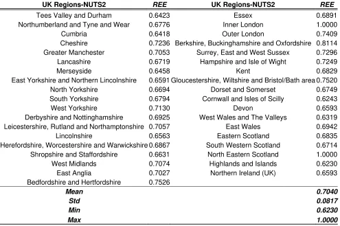
The empirical results (Table1) indicate that Inner London and North Eastern

Scotland appear to be environmental efficient regions. In addition the last fiveUK

regions in terms of the lowest environmental efficiencies are reported to be Tees

Valley and Durham, Cumbria, West Wales and The Valleys, Cornwall and Isles of

Scilly and Highlands and Islands. In addition Table 1 indicates that the average REE

level is 0.7 (with standard deviation equals to 0.09). As it can be observed only

fourteen UK regions are reported to have REE score above 0.7. These are reported to

be Inner London, North Eastern Scotland, Berkshire, Buckinghamshire and

Oxfordshire, Bedfordshire and Hertfordshire, Gloucestershire, Wiltshire and

Bristol/Bath area, Outer London, Surrey, East and West Sussex, Hampshire and Isle

of Wight, Cheshire, West Yorkshire, West Midlands, Leicestershire, Rutland and

Northamptonshire, Greater Manchester and East Anglia.

7

[image:8.595.52.547.106.435.2]

Table 1: UK regions’ environmental efficiency levels measured in Shephard’s output distance functions

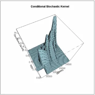
Furthermore, and in order to understand how per capita regional income levels

affect regions environmental efficiencies we construct conditional stochastic kernels

between REE and GDPPC variables8. This relationship is presented on Figure 1 in a

conditional stochastic kernel form. When looking Figure 1 we can choose a fixed

point on the axis labeled REE and then by slicing the graph from this point and

moving parallel to GDPPC axis, the estimated distribution of regions’ REE levels

over the examined time period conditional on GDPPC levels can be traced. The

graphic shows that regions in the extremes of environmental efficiency have higher

probability which have been generated by the respective extremes of per capita

8

The routes and theory behind the link of environmental quality and economic development stages, income disparities can be found in the works of Kuznets (1955), Grossman and Kruger (1995) and Dasgupta et al. (2002).

UK Regions-NUTS2 REE _{UK Regions-NUTS2} REE

Tees Valley and Durham 0.6423 Essex 0.6891

Northumberland and Tyne and Wear 0.6776 Inner London 1.0000

Cumbria 0.6418 Outer London 0.7409

Cheshire 0.7236 Berkshire, Buckinghamshire and Oxfordshire 0.8114 Greater Manchester 0.7053 Surrey, East and West Sussex 0.7296

Lancashire 0.6719 Hampshire and Isle of Wight 0.7249

Merseyside 0.6458 Kent 0.6829

East Yorkshire and Northern Lincolnshire 0.6591 Gloucestershire, Wiltshire and Bristol/Bath area 0.7520

North Yorkshire 0.6694 Dorset and Somerset 0.6749

South Yorkshire 0.6794 Cornwall and Isles of Scilly 0.6243

West Yorkshire 0.7130 Devon 0.6593

Derbyshire and Nottinghamshire 0.6925 West Wales and The Valleys 0.6319 Leicestershire, Rutland and Northamptonshire 0.7057 East Wales 0.6942

Lincolnshire 0.6563 Eastern Scotland 0.6835

Herefordshire, Worcestershire and Warwickshire 0.6867 South Western Scotland 0.6714 Shropshire and Staffordshire 0.6631 North Eastern Scotland 1.0000

West Midlands 0.7074 Highlands and Islands 0.6230

East Anglia 0.7027 Northern Ireland (UK) 0.6593

Bedfordshire and Hertfordshire 0.7526

Mean 0.7040

Std 0.0817

Min 0.6230

growth levels. That is low-environmental efficiency regions have high probability that

have been generated by lower GDP per capita levels and high-environmental

efficiency regions, by higher GDP per capita levels. However, for the

intermediate-environmental efficient regions (with REE between 0.65-0.70), the effect of per capita

income is less determinant, given the high dispersion of estimated densities. We can

[image:9.595.125.435.295.606.2]

interpret this result as club convergence (which is conditioned on GDPPC)9.

Figure 1: Conditional stochastic kernels of UK regions-Regional environmental efficiency (REE) conditioned on regional GDP per capita (GDPPC) levels

Finally, in respect to the methodologies adopted the contribution of the paper

is twofold: to demonstrate how directional distance functions can be applied in a

regional level and how then the estimation of conditional stochastic kernels can be

9

used in order to examine the regional environmental quality-economic growth

References

Chung Y.H., Färe R., Grosskopf S., 1997. Productivity and undesirable outputs: A directional distance function approach. Journal of Environmental Management 51, 229– 240.

Dasgupta S., Laplante B., Wang H., Wheeler D. 2002. Confronting the Environmental Kuznets Curve. Journal of Economic Perspectives 16, 147– 168.

Färe R., Grosskopf S., Tyteca D. 1996. An activity analysis model of the environment performance of firms: application to fossil-fuel-fired electric utilities. Ecological Economics 18, 161–175.

Färe R., Grosskopf S. 2003. Non-parametric Productivity Analysis with Undesirable Outputs: Comment. American Journal of Agricultural Economics 85, 1070–74.

Färe R., Grosskopf S. 2009. A Comment on Weak Disposability in Nonparametric Production Analysis. American Journal of Agricultural Economics 91, 535-538.

Färe, R., Grosskopf, S., Lovell, C.A.K., Pasurka, C., 1989. Multilateral productivity comparisons when some outputs are undesirable. The Review of Economics and Statistics 71, 90–98.

Färe R., Primont D. 1995. Multi-Output Production and Duality: Theory and Applications. Kluwer Academic Publishers, Boston.

Färe R., Grosskopf S. 2004. Modeling undesirable factors in efficiency evaluation: Comment. European Journal of Operational Research 157, 242-245.

Fotopoulos G. 2006. Nonparametric analysis of regional income dynamics: The case of Greece. Economics Letters 91, 450-457.

Grossman G.M., Krueger A.B. (1995) Economic growth and the environment. The Quarterly Journal of Economics 110, 353-377.

Hailu A. 2003. Non-parametric Productivity Analysis with Undesirable Outputs: Reply. American Journal of Agricultural Economics 85, 1075–77.

Hailu A., Veeman TS. 2001. Non-parametric Productivity Analysis with Undesirable Outputs: An Application to the Canadian Pulp and Paper Industry. American Journal of Agricultural Economics 83, 605–16.

Hall P., Racine J.S., Li Q. 2004. Cross-validation and the estimation of conditional probability densities. Journal of the American Statistical Association 99, 1015–1026.

Kuosmanen T., Podinovski V. 2009. Weak disposability in nonparametric production analysis: reply to Färe and Grosskopf. American Journal of Agricultural Economics 91, 539-545.

Kuznets S. 1955. Economic growth and income inequality. American Economic Review 45, 1-28.

Poletti Laurini M., Valls Pereira P.L. 2009. Conditional stochastic kernel estimation by nonparametric methods. Economics Letters 105, 234-238.

Racine J.S. 2008. Nonparametric Econometrics: A Primer. Found and Trends Econometrics 3, 1-88.

Shephard R.W. 1970. Theory of Cost and Production Functions. Princeton University Press, Princeton, NJ.

Shephard R.W., Färe R. 1974. The law of diminishing returns. Zeitschrift für Nationalökonomie 34, 60–90.

Tyteca D. 1996. On the Measurement of the Environmental Performance of Firms- A Literature Review and a Productive Efficiency Perspective. Journal of Environmental Management 46, 281- 308.

Tyteca D. 1997. Linear programming models for the measurement of environmental performance of firms: concepts and empirical results. Journal of Productivity Analysis 8, 175–189.

Zelenyuk V., Zheka V. 2006. Corporate governance and firm’s efficiency: the case of a transitional country, Ukraine. Journal of Productivity Analysis 25, 143-157.