Estimating NAS Consistent Poverty and Inequality from NSS Data

Estimating NAS Consistent Poverty and

Inequality from NSS Data

Chaganti, Ravi and Motkuri, Venkatanarayana

Centre for Economics and Social Studies, Hyderabad

February 2011

1

Estimating NAS Consistent Poverty and Inequality from NSS Data

*

C. Ravi and M. Venkatanarayana

I Introduction

Poverty alleviation has become an important Plan objective and successive plans have been specifying the poverty alleviation targets in India. Ever since the issues of poverty gained the policy attention in the development planning, there exists diversity of opinion among experts on the methodology of measuring poverty. There are multiple dimensions of poverty. However, the base for the income poverty estimations in India has been the consumption expenditure but the estimates of consumption expenditure are generated from the two sources. The first source is the CSO, as a part of the National Accounts and Statistics (NAS) it compiles annually the estimates of private final consumption expenditure (PFCE). The second source is the Household Consumption Expenditure Survey based estimates of National Sample Survey Organisation (NSSO). The concern is that estimates from these two sources are not made to reconcile with each other, rather the divergence between the two sources has been increasing. It is well established fact that the NSS consumption expenditure survey based estimate has always been lower than that of NAS.

The factors of difference in estimates of consumption expenditure by these two sources are already acknowledged (CSO, 2008; Sundaram and Tendulkar, 2001 & 2003). The major explicit difference between the two sources of estimates of aggregate consumption expenditure is the coverage. There are factors like methods, prices and imputations of notional elements etc., which contribute to the difference between the two sources (see CSO, 2008; Sundaram and Tendulkar, 2001 & 2003).

However, the increasing divergence between the two sources raised the argument that NSS estimates are missing a part of the total consumption expenditure so that it is an under estimate (Bhalla, 2007 & 2010). The difference between the two sources of consumption expenditure also led to the counter evidence of a lower estimate of poverty ratios based NAS consumption to that of Planning Commissions’ official estimate of poverty ratio based on NSS consumption expenditure data. An extreme argument put forwarded is that India has already reached poverty related Millennium Development Goal (Bhalla, 2003). The controversial evidence of lower

*

Draft Paper presented at Annual Conference of Indian Association Income and Wealth Research (IAIWR) held at CESS, Hyderabad during 11-12 February, 2011.

# _{The first author is a Faculty and the second author is a Research Consultant at Centre for Economic and}

2 poverty ratio has generated debate on comparison of NAS and NSS based estimations (See Bhalla 2003, 2007 & 2010; Ravallion, 2000 & 2003; Sundaram and Tendulkar, 2001 & 2003).

In this context it is an attempt to make the estimates of poverty and inequality consistent with NAS based consumption expenditure (PFCE) from NSSO based consumption expenditure data. It is to be noted that the paper is not going address the poverty measurement controversy based on two sources of estimations but explores consistent estimation. Having said, the content of the paper is organized as follows. The second section presents the divergence between the NAS and NSS estimates of aggregate consumption expenditure and the factors that contributes to the difference. In the third section an analysis of divergence factor across per capita expenditure fractile (5% population) classes is presented. The fourth section presents an estimation of NAS’s PFCE consistent poverty and inequality from NSS’s consumption expenditure data. The last section finally summarises the content and concludes.

II Increasing Divergence between NSS and NAS Estimates

It is observed that the difference between the aggregate Household Consumption Expenditure (HCE) of NSS and the aggregate Private Final Consumption Expenditure (PFCE) of NAS has been widening over a period (Table 1). The However, the difference between NSS and NAS in expenditure on food is lower than that of the non-food items.

Table 1 : Divergence in Estimates of Aggregate

Consumption Expenditure (in Rs. Cr.) in India between NSS and NAS

Year (NSS)

NSS Reference

NAS Base

Food Non-Food All Difference (in %) NSS NAS NSS NAS NSS NAS Food

Non- Food All

1 2 3 4 5 6 7 8 9 10 11 12

1972-73 URP 1970-71 23420 23379 9790 11752 33210 35131 0.18 -16.70 -5.47 1977-78 URP 1970-72 36500 39801 20030 23282 56530 63083 -8.29 -13.97 -10.39 1983 URP 1980-81 69735 85613 39996 60471 109731 146084 -18.55 -33.86 -24.88 1987-88 URP 1980-82 106205 122805 67560 101256 173765 224061 -13.52 -33.28 -22.45 1993-94 URP 1993-94 224066 315243 131704 259529 355770 574772 -28.92 -49.25 -38.10 1999-00 URP 1993-94 393126 652627 323265 618929 716391 1271556 -39.76 -47.77 -43.66 1999-00 URP 1999-00 410918 647011 305473 610530 716391 1257541 -36.49 -49.97 -43.03 2004-05 URP 1999-00 481189 742609 450226 1131120 931415 1873729 -35.20 -60.20 -50.29 2004-05 MRP 1999-00 481189 742609 485204 1131120 966393 1873729 -35.20 -57.10 -48.42

Note: URP – Uniform Reference Period (30 Days); MRP – Mixed Reference Period (30 and 365 Days); 2. Current Prices.

Source: CSO (2008).

3 only to consumption expenditure in the household sector and thus excludes the non-household sector (i.e. houseless, institutional, non-governmental, non-profit institutions serving households (NPISH), etc.) whereas the NAS estimates are based broader coverage including both the household and non-household sectors.

The other major difference is that NAS’s consumption expenditure (PFCE) estimates are based commodity flow approach whereas the NSS estimates are actual consumption expenditure during the one year survey reference period.

Thirdly, the NAS estimate of private final consumption expenditure (PFCE) includes two notional elements such as imputed rents on owner-occupied dwellings and financial intermediation services indirectly measured1 (FISIM). Another factor that contributes the difference is reported prices of commodities at purchase in the survey and imputed prices used to estimate the value of consumption by NAS.

In order obtain an estimate comparable (between NAS and NSS) in coverage the information on consumption expenditure of NPISH, houseless and an institutional population is not available separately. Thus we cannot either net out from the estimate PFCE of NAS or add to the household consumption expenditure of NSS. Although the proportion of consumption expenditure related houseless and institutional population in PFCE could be very small, the share of NPISH is expected to be significantly high and rising over time with increasing roles of various NGOs in different sector especially in health and education (Sundaram and Tendulkar, 2003). With respect to the notional elements of imputed rent and FISIM, information on its estimate is available with NAS so that it can be netted out (Sundaram and Tendulakar, 2003).

Having observed discrepancies an attempt is made to reduce the difference between the two sources estimates by eliminating discrepancy factors. In this regard, firstly of all, the consumption expenditure related to rent (both actual and imputed) is excluded from both the source of estimates. Secondly, the value of FISIM embedded especially with the estimates of consumption expenditure related to ‘Miscellaneous Good and Services’ commodity group is excluded.

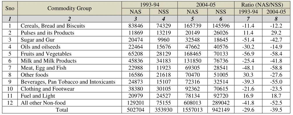
Table 2 presents the aggregate consumption expenditure in India by broad commodity group estimated from both the NAS and NSS. The concordance of commodity group between NSS and NAS is done using CSO’s Source and Methods of NAS and its report: Report of The Group for Examining Discrepancy in PFCE Estimates from NSSO Consumer Expenditure Data and Estimates Compiled by National Accounts Division (CSO, 2008). For the PFCE estimates of NAS (current prices) by standard detailed commodity groups is taken from CSO website for the years 1993-94 and 2004-05 to match with NSS 50th and 61st rounds Survey on household consumption expenditure and collapsed the standard detailed commodity grouping values into broad commodity grouping (see Table 2). The corresponding commodity grouping is made in the NSS 50th and 61st rounds Consumption Expenditure Survey using unit record data. NSS estimates of consumption expenditure are based on MRP (30 and 365 days) data. These

1

4 estimates exclude the values of consumption expenditure related to rent (actual as well as imputed) and values of FISIM.

Table 2: Divergence in Estimates of Aggregate Consumption Expenditure (Rs. Cr.) in India between NSS and NAS by Commodity Groups

Sno Commodity Group 1993-94 2004-05 Ratio (NAS/NSS) NAS NSS NAS NSS 1993-94 2004-05

1 2 3 4 5 6 7 8

1 Cereals, Bread and Biscuits 83846 74329 165739 145596 -11.4 -12.2 2 Pulses and its Products 11869 13219 20149 26026 11.4 29.2 3 Sugar and Gur 20474 9960 32548 18645 -51.4 -42.7 4 Oils and oilseeds 22464 15676 47662 40576 -30.2 -14.9 5 Fruits and Vegetables 65208 28129 168465 70133 -56.9 -58.4 6 Milk and Milk Products 45836 34183 131850 76736 -25.4 -41.8 7 Meat, Egg and Fish 22988 11923 69305 28541 -48.1 -58.8 8 Other foods 16586 21618 70470 51005 30.3 -27.6 9 Beverages, Pan Tobacco and Intoxicants 24873 15107 72316 32514 -39.3 -55.0 10 Clothing and Footwear 38380 30105 92362 70615 -21.6 -23.5 11 Fuel and Light 20979 24527 78134 92720 16.9 18.7 12 All other Non-food 129201 75155 608013 289042 -41.8 -52.5 Total 502704 353930 1557013 942149 -29.6 -39.5

Note: 1. NSS estimates are based MRP data; 2. Current Prices; 3. For NAS the base is 1999-2000.

Source: 1. CSO for NAS Estimates; 2. NSS 50th and 61st Consumption Expenditure Survey raw data.

It is observed that the exclusion of values of notional elements (rent and FISIM) reduced the overall difference between NAS and NSS, about 10 percentage points in both the time points (1993-94 and 2004-05). When one observes the commodity group wise difference between NAS and NSS in estimates of consumption expenditure, for the two commodity groups, pulses and its products together and fuel and light, NSS estimates of consumption expenditure are higher than that of NAS. In all other commodity groups NAS estimates are higher than NSS. Among the food related commodity groups, the difference between NAS and NSS in consumption expenditure is very high from meat, egg and fish group; the lowest difference is observed from Cereal, Bread and Biscuits group.

The discrepancy in the estimate of overall aggregate consumption expenditure or by commodity group wise, from the two different sources of estimations can be addressed once the two sources comparable in coverage wherein information on the proportion of non-household sector especially the NPISH is made available.

III Increasing Divergence between NSS and NAS Estimates by Fractiles

5 based on the NSS consumption expenditure survey unit record data. Then a matrix of 20 fractile classes and 37 broad commodity group (in concordance with NAS) generated for rural and urban sector wherein the aggregate consumption expenditure in each fractile class is derived for each broad commodity group and subsequently the per capita expenditure for each commodity group for each fractile is derived. NSS consumption expenditure for 30 days is annualized by multiplying 365 (days) but not 12 (months).

Similarly the sector, fractile class, and broad commodity wise distribution of per capita consumption expenditure of NAS based PFCE is also derived using the following method.

NASPFCE (A, j)

PCPFCENAS(R, i, j) = --- X PCCENSS(R, i, j) --- (1)

(NSSCE(R, j) + NSS CE (U, j))

NASPFCE (A)

PCPFCENAS (U, i, j) = --- X PCCENSS (U, i, j) --- (2)

(NSSCE(R, j) + NSSCE (U, j))

Fractile Class - i = 1, 2,….., 20 (total 20 fractile classes)

Broad Commodity Group - ‘j’ = 1, 2, ……, 37 (total 37 commodity groups)

Sector: A – All/Aggregate (rural and urban) R – Rural; U - Urban

Sources: NAS – National Accounts and Statistics; NSS – National Sample Survey

Per Capita: PCPFCE – Per Capita Private Final Consumption Expenditure; PCCE – Per Capita Consumption Expenditure

Aggregate: PFCE - Private Final Consumption Expenditure; CE – Consumption Expenditure

While distributing the commodity group specific per capita consumption expenditure of NAS based PFCE across fractiles and the sector, the above method takes the variation in commodity specific difference factor (ratio of NAS/NSS) as it is, but assumes same commodity specific difference factor across fractile classes and sector (rural and urban).

6 broad commodity wise per capita consumption expenditure is aggregated across fractiles in each sector.

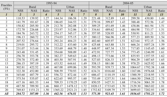
Table 3 presents fractile wise mean per capita consumption expenditure by sector (rural and urban) and by source of consumption expenditure estimation (NAS and NSS) and for two points of time (1993-94 and 2004-05) and the difference factor (the ratio of NAS/NSS) across fractiles. This difference factor is also shown graphically in Figure 1 and 2.

Table 3: Difference between NSS and NAS

in Monthly Per Capita Consumption Expenditure in India by PCE Fractile Classes

Fractiles (5%)

1993-94 2004-05

Rural Urban Rural Urban

NSS NAS Ratio NSS NAS Ratio NSS NAS Ratio NSS NAS Ratio

1 2 3 4 5 6 7 8 9 10 11 12 13

1 110.53 139.92 1.27 144.34 186.58 1.29 221.48 312.89 1.41 299.58 430.80 1.44 2 141.79 181.67 1.28 186.65 244.53 1.31 279.16 399.87 1.43 388.48 572.56 1.47 3 158.82 205.50 1.29 212.78 282.08 1.33 309.25 451.69 1.46 438.86 661.94 1.51 4 172.70 226.68 1.31 233.97 312.06 1.33 334.61 489.62 1.46 484.98 733.17 1.51 5 184.76 243.72 1.32 254.17 345.17 1.36 357.95 528.95 1.48 530.91 811.21 1.53 6 196.13 260.72 1.33 274.03 375.15 1.37 380.12 566.96 1.49 577.23 889.50 1.54 7 207.52 276.64 1.33 292.24 404.23 1.38 402.60 605.97 1.51 623.64 972.15 1.56 8 219.01 295.72 1.35 312.22 433.60 1.39 425.68 643.88 1.51 666.24 1057.24 1.59 9 231.07 313.44 1.36 333.69 468.79 1.40 448.97 687.34 1.53 717.85 1145.45 1.60 10 243.48 331.45 1.36 354.68 508.09 1.43 472.91 727.77 1.54 773.45 1246.99 1.61 11 256.70 353.78 1.38 382.27 549.63 1.44 498.13 773.66 1.55 835.93 1357.55 1.62 12 270.78 372.40 1.38 403.50 587.91 1.46 527.03 826.33 1.57 904.29 1487.65 1.65 13 286.15 397.19 1.39 433.52 644.61 1.49 558.13 881.00 1.58 978.25 1625.92 1.66 14 302.81 422.52 1.40 467.00 699.06 1.50 593.59 939.73 1.58 1064.67 1792.38 1.68 15 322.30 452.00 1.40 508.59 770.93 1.52 634.31 1016.60 1.60 1167.06 1976.68 1.69 16 345.60 487.79 1.41 556.72 872.44 1.57 686.47 1110.19 1.62 1300.39 2218.95 1.71 17 375.54 535.07 1.42 622.65 995.57 1.60 753.49 1237.51 1.64 1464.50 2568.22 1.75 18 417.16 601.33 1.44 709.33 1170.25 1.65 850.55 1427.31 1.68 1716.54 3061.39 1.78 19 487.50 709.50 1.46 860.17 1478.12 1.72 1020.13 1733.65 1.70 2129.30 3863.02 1.81 20 769.83 1151.21 1.50 1365.22 2521.21 1.85 1752.82 3109.79 1.77 3699.03 7202.93 1.95

All 284.72 387.00 1.36 442.56 676.81 1.53 575.30 923.43 1.61 1036.65 1781.23 1.72

Note: PCE - Per Capita Expenditure.

Source: Authors estimates based on CSO’s NAS estimates and NSS 50th and 61st Consumption Expenditure Survey raw data.

7 Figure 1: Ratio (NAS/NSS) of Mean Monthly Per Capita Consumption Expenditure across

Fractile Classes: India, 1993-94

Figure 2: Ratio (NAS/NSS) of Mean Monthly Per Capita Consumption Expenditure across Fractile Classes: India, 2004-05

1.00 1.10 1.20 1.30 1.40 1.50 1.60 1.70 1.80 1.90

1 2 3 4 5 6 7 8 9 10 11 12 13 14 15 16 17 18 19 20

R

at

io

Fractile Classes

Rural Urban

1.00 1.10 1.20 1.30 1.40 1.50 1.60 1.70 1.80 1.90 2.00

1 2 3 4 5 6 7 8 9 10 11 12 13 14 15 16 17 18 19 20

R

at

io

Fractile Classes

8 IV Inequality and Poverty

When observed the growth of real MPCE during last one decade period between 199394 and 2004-05, NAS based MPCE has shown a very high growth than that of the NSS based MPCE; in fact, NAS based MPCE is grown double the times the growth that NSS based MPCE has shown especially in rural sector (see Table 4).

Table 4: Growth of MPCE and Change in Inequality

Year

Rural Urban NSS NAS NSS NAS

1 2 3 4 5

MPFCE in 1993-94 Prices 1993-94 284.7 387.0 442.6 676.8 2004-05 328.6 527.5 545.8 937.9 % Change 15.43 36.31 23.34 38.57

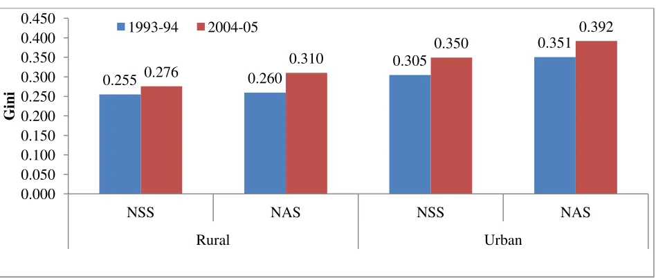
Inequality - Gini 1993-94 0.255 0.260 0.305 0.351 2004-05 0.276 0.310 0.350 0.392 % Change 8.03 19.43 14.73 11.72

Note:

Source: Authors Estimations

Based on the information furnished in the Table 3, Gini Coefficients are derived for NAS and NSS based MPCEs and by sectors, to indicate the level of inequality (see Table 4 and Figure 3). It is noted that NAS consumption expenditure distribution has shown higher Gini value than that of NSS in both the rural and urban sectors.

Figure 3: Gini Coefficients

0.255 0.260

0.305

0.351

0.276 0.310

0.350

0.392

0.000 0.050 0.100 0.150 0.200 0.250 0.300 0.350 0.400 0.450

NSS NAS NSS NAS

Rural Urban

G

in

i

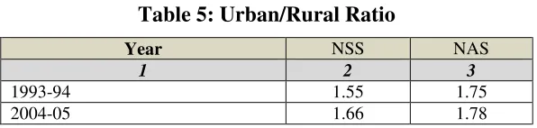
9 Table 5: Urban/Rural Ratio

Year NSS NAS

1 2 3

1993-94 1.55 1.75 2004-05 1.66 1.78

Source: Calculated from Table 3.

The rural-urban ratio in terms of MPCE shows that the urban MPCE is more than 1.5 times more than the rural MPCE (Table 5). The ratio is observed to be higher in NAS based MPCE when compared to NSS based MPCE. Moreover it has increased between 1993-94 and 2004-05 indicating increasing rural-urban divide.

Poverty

Given the poverty line, for estimating number of poor the practice of Planning Commission by its ‘Official Methodology’ especially during 1970s and 1980s was that it used adjust the NSS data to anchor it with NAS estimate of aggregate consumption expenditure.

The following extract from the Planning Commission’s Report of the Expert Group on Estimation of Proportion and Number of Poor (known as Lakdwala Committee Report) 1993, elicits the adjustment procedure for estimating population below poverty line according to official methodology was as following:

“In order to arrive at the estimates of the number of poor, Planning Commission has been making adjustment in the National Sample Survey (NSS) data on distribution of households by consumption expenditure levels. Such an adjustment has been felt to be necessary because the aggregate private household consumption expenditure as estimated from the NSS data is different from the aggregate private consumption expenditure estimated in the National Accounts Statistics (NAS). It was considered desirable to have compatibility between the two sets of data in order to

ensure consistency between the two important components of the plan model, i.e., the

input-output table (based on NAS) and consumption sub-model (based on NSS data). The procedure followed has been to adjust the expenditure levels reported by the NSS uniformly across all expenditure classes by a factor equal to the ratio of the total private consumption expenditure obtained from the NAS to that obtained from the NSS. The old NAS series was used for deriving the adjustment factor for the estimates up to year 1983 and the new NAS series has been used for

the 1987-88 estimates.”(Planning Commission, 1993).

Thus the population below poverty line used to be estimated:

“….by applying the updated poverty line to the corresponding adjusted NSS distribution of households by levels of consumption expenditure. To estimate the incidence of poverty at the State level, all-India poverty lines and the adjustment factors have been used on the State specific NSS distribution of households by levels of consumption expenditure uniformly across the

10 Having observed the problems involved with the pro-rata adjustment of NSS expenditure class distribution to anchor with NAS’ estimate of aggregate consumption expenditure by raising the NSS consumption expenditure level across expenditure classes by a factor equal to the ratio of the aggregate consumption expenditure of NAS and that of NSS, the Expert Group (Lakdawala Committee) preferred to estimate the incidence of poverty entirely based on the NSS consumption expenditure survey data. The following extract from its report elicits the same.

“The Planning Commission has in the past "adjusted" the frequency distribution derived from the NSS for the discrepancy between the NSS and the national accounts based estimates put out by CSO of the aggregate consumption expenditure (pee). This adjustment is made on the assumption that the difference between the two estimates of mean pee at the national level is distributed uniformly across States, and across all sections of the population. We do not find this procedure acceptable because it involves arbitrary pro- rata adjustment in the distribution. Under the circumstances it is better to rely exclusively on the NSS for estimating the poverty ratio by State and in rural and urban areas.”(Planning Commission, 1993).

However, one cannot out rightly deny the compatibility of the estimate of consumption expenditure from these two different sources. As the Expert Group itself admitted its report, it is desirable to have compatibility between the two sets of data in order to ensure consistency between the two important components of the plan model, i.e., the input-output table (based on

NAS) and consumption sub-model (based on NSS data). Taking this an exercise for deriving NAS consistent poverty ratio from NSS consumption expenditure data is taken up. Table 6 presents the preliminary results of the exercise.

The NAS adjusted Poverty Lines and Poverty Ratios (Head Count Ratio) are based on the Lorenz Curve equation. The NAS poverty line is derived by taking the Tendulkar Committee’s NSS (MRP) based poverty line for the year 2004-05 and corresponding poverty ratio (HCR),

ZNSS (2004-05) => HCRNSS (2004-05) => £NAS (2004-05) => ZNSS (2004-05)

Z = Poverty Line

HCR = Head Count Ratio

£ = Distribution

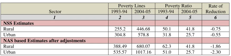
11 Table 6: Poverty Line and Head Count Ratios, India

Sector

Poverty Lines Poverty Ratio Rate of Reduction 1993-94 2004-05 1993-94 2004-05

1 2 3 4 5 6

NSS Estimates

Rural 255.2 446.68 50.1 41.8 -0.75 Urban 304.8 578.8 31.8 25.7 -0.55

NAS based Estimates after adjustments

Rural 388.49 680.07 62.3 41.8 -1.86 Urban 535.57 1017.16 51.0 25.7 -2.30

Note: Estimates after adjustments – are NAS Consistent.

Source: Authors Estimates.

It can be observed that the levels of poverty varies by the sources of estimates of consumption expenditure but the change (rate of reduction) during the one decade period between 1993-94 and 2004-05 is faster according to the NAS’s estimate of consumption expenditure.

V Summary and Conclusions

The present paper made an attempt for estimating of NAS’s PFCE consistent poverty and inequality from NSS’s consumption expenditure data. Taking note of the increasing divergence in estimates of aggregate consumption expenditure between two important sources: NAS and NSS, redistributed the MPCE across 20 fractile classes and observed that the difference factor is increasing along with fractile class.

* * *

References

Bhalla, Surjit (2002) Imagine There’s No Country: Poverty, Inequality and Growth in the Era of

Globalisation, Institute of International Economics.

Bhalla, Surjit (2003) “Crying Wolf on Poverty: Or How the Millennium Development Goal for Poverty

Has Already Been Reached”, Economic and Political Weekly, 5th July.

Bhalla, Surjit (2007) “World Bank – Peddling Poverty”, Business Standard, December 22, 2010.

Bhalla, Surjit (2010) “India’s Real Povery”, Business Standard, January 9, 2010.

CSO (2008) Report of The Group for Examining Discrepancy in PFCE Estimates from NSSO

Consumer Expenditure Data and Estimates Compiled by National Accounts Division, Central Statistical Organisation, Ministry of Statistics and Programme Implementation, Government of India.

12 Minhas, B S (1988) “Validation of Large Scale Sample Survey Data: A Case of NSS Estimates of

Household Consumption Expenditure”, Sankhya, A, Series B, Vol. 50.

Minhas, B. S. and S. M. Kansal (1989) “Comparision of NSS and CSO Estimates of Private

Consumption: Some Observations Based on 1983 Data”, The Journal of Income and Wealth, Vol.

11 (1), January.

Planning Commission (1993) Report of the Expert Group on Estimation of Proportion and Number

of Poor, Perspective Planning Division, Planning Commission, Government of India, New Delhi.

Ravallion, Martin (2000) “Should Poverty Measures Be Anchored to the National Accounts?”, Economic

and Political Weekly, 2nd August.

Ravallion, Martin (2003) “Fanciful Numbers and Fictious Intrigues”, Economic and Political Weekly, 1st

November.

Sundaram, K. and Suresh D. Tendulkar (2001) “NAS-NSS Estimates of Private Consumption for Poverty

Estimation: A Disaggregated Comparison for 1993-94”, Economic and Political Weekly, 13th

January.

Sundaram, K. and Suresh D. Tendulkar (2003) “NAS-NSS Estimates of Private Consumption for Poverty