Selecting between different productivity measurement approaches: An application using EU KLEMS data

Munich Personal RePEc Archive

Selecting between different productivity

measurement approaches: An application

using EU KLEMS data

Giraleas, Dimitris and Emrouznejad, Ali and Thanassoulis,

Emmanuel

Aston Business School, Aston University

March 2012

Online at

https://mpra.ub.uni-muenchen.de/37965/

Selecting between different productivity

measurement approaches: An application

using EU KLEMS data

Dimitris Giraleas

_{, Ali Emrouznejad and Emmanuel Thanassoulis}

Operations and Information Management, Aston Business School, Aston University, Birmingham, UK

Abstract: Over the years, a number of different approaches were developed to measure productivity change, both in the micro and the macro setting. Since each approach comes with its own set of assumptions, it is not uncommon in practice that they produce different, and sometimes quite divergent, productivity change estimates. This paper introduces a framework that can be used to select between the most common productivity

measurement approaches based on a number of characteristics specific to the application/dataset at hand; these were selected based on the results of previous simulation analysis that examined the accuracy of different

productivity measurement approaches under different conditions. The characteristics in question include input volatility through time, the extent of technical inefficiency and noise present in the dataset and whether the parametric approaches are likely to suffer from functional form miss-specification and are examined using a number of well-established

diagnostics and indicators. Once assessed, the most appropriate approach can be selected based on its relative accuracy under these conditions;

accuracy can in turn be assessed using simulation analysis, either previously published or designed specifically to emulate the characteristics of the

application/dataset at hand. As an example of how this selection framework can be implemented in practice, we assess the productivity performance of a number of EU countries using the EU KLEMS dataset.

Keywords: Data envelopment analysis, Productivity and competitiveness, Simulation, Stochastic Frontier Analysis, Growth accounting

1

2

1 Introduction

Increasing productivity is of paramount importance to policy makers in both the micro (ie company-level) and macro (ie industry- and economy-level) settings, since productivity growth leads to increased prosperity both in the short term and long-run. In fact, according to neoclassical theory, productivity growth is the only sustainable source of growth in the long-run since factor accumulation provides only decreasing returns to growth (Solow, 1957). Given the importance of productivity growth in both the micro but especially in the macro level, where increasing input utilisation is more difficult, it is critical for policy makers to accurately measure its progress. Accurate measures of productivity change are a necessary requirement for any analysis that looks for the likely drivers of productivity growth; once these drivers are identified, policy makers can work on fostering the development of such drivers in the economy, leading to increased economic prosperity.

There are a number of approaches that could be used to measure productivity change, both in the macro (ie economy- or industry-wide) and micro (eg

company or department) level, and each has its own strengths and

weaknesses (Knox Lovell, 1996). Usually, the analysis will adopt more than one of these approaches, so that comparisons between the different

productivity change estimates are possible (see for example (Odeck, 2007)).

It is not uncommon in such applications that the different approaches result in different estimates; in some cases, these differences can be quite substantial (Coelli, 2002). In those instances, the analysis would need to be able to put forward an informed view on why the various approaches come up with such divergent views and, more importantly, which estimates are likely to be more accurate. The aim of this paper is to suggest a framework which could be used to select between the competing estimates, based on the likely accuracy of the adopted approaches when taking into account the

To develop this framework, we heavily rely on the simulation experiments undertaken in Giraleas et al.2 _{(forthcoming) (referred to from now on as GET),}

which examined the overall accuracy of some of the most commonly-used productivity measurement approaches under a number of different conditions. The experiments revealed that the relative accuracy of each approach heavily depends on said conditions; therefore, if we could identify which

characteristics/conditions are prevalent in the application/dataset currently examined, we could use the simulation evidence to select the productivity estimates that are likely to be more accurate. This paper proposes a set of readily available diagnostic tests and/or indicators that could be used to asses the aforementioned conditions/characteristics; when combined, these

diagnostic tests and indicators would constitute the selection framework. The application of this framework is demonstrated using the EU KLEMS dataset (EU KLEMS, 2008).

The paper is structured as follows. Section 2 presents the selection framework and how it can be applied in practice. Section 3 assesses the annual productivity change for a group of countries by a number of approaches, using the EU KLEMS dataset, and compares the resulting estimates. Section 4 demonstrates an application of the selection framework using the analysis in section 3 as an example. Lastly, section 5 provides a summary of the selection framework and concludes.

2

Selection framework in the macro setting

Productivity change in the macro setting (aggregate productivity) is usually measured utilising a single measure of aggregate output (usually expressed in value added terms) and a limited number of aggregate inputs (labour and capital if output is measured in value added terms). The most common approach of measuring aggregate productivity change is growth accounting (GA). Probably the largest contributor to the wide adoption of GA amongst policy makers is that GA estimates can be (relatively) easily produced using country- or sector-specific National Accounts data, without recourse to information from outside the country or the sector examined; on the other hand, GA requires the adoption of a number of, potentially unrealistic

2

4

assumptions, most notably those relying on the existence of perfect competition, which could lead to unreliable estimates (for a more detailed discussion see section 3.2).

Frontier-based approaches can also be used to estimate productivity change and unlike GA, they do not rely on the (restrictive) assumptions of perfectly competitive markets nor do they require information on prices. On the other hand, frontier-based approaches require information on comparators, so they are, in a sense, more data intensive than GA. The most common frontier-based approaches for measuring productivity change are Data Envelopment Analysis (DEA), Corrected Ordinary Least Squares (COLS) and Stochastic Frontier analysis; these are also the focus of this paper and are discussed in more detail in section 3.2.

In terms of the overall accuracy of each approach, the simulation analysis undertaken in GET demonstrated that no single approach has an absolute advantage over another; rather, their relative accuracy depends on the characteristics of the data generating process (DGP), or, in other words, the characteristics of the application/dataset at hand.

2.1 Characteristics of interest

The simulation analysis undertaken in GET revealed that the most influential characteristics of the DGP to the accuracy of the examined approaches are:

– the extend of volatility in inputs from one year to the next. Increased volatility adversely affects the accuracy of all approaches, but DEA-based estimates are the least affected, while the GA estimates are the most affected;

– the extend of inefficiency present in the sample. Increased levels of technical inefficiency have only a small negative effect on the accuracy of COLS- and DEA-derived productivity estimates, but a larger impact on GA and SFA-based estimates (for the SFA estimates the change in accuracy is co-dependent on the extend of measurement error-noise in the data);

and on whether the parametric approaches are likely to suffer from functional form miss-specification;

– whether the parametric approaches are likely to suffer from functional form miss-specification; Functional form misspecification has a severe negative impact on the accuracy of all parametric approaches.

The first step of the proposed selection framework is to assess how prevalent the above characteristics are (if at all) in the application/dataset at hand. This assessment is not straightforward; in fact, it is impossible to determine with certainty at least some of the characteristics in question, given that all productivity measurement approaches examined rely on certain implicit or explicit assumptions, which are made prior to the actual analysis, that directly influence the estimates used to assess said characteristics. For example, both COLS and DEA are so-called ‘deterministic approaches’, meaning that they assume that there is no measurement error/noise in the sample data. Another example is that most frontier-based approaches automatically assume that there is some inefficiency (SFA is the exception, as it can test for the

presence inefficiency), while GA assumes that there is no inefficiency in the sample data.

Despite the above concerns, there are a number of simple diagnostic tests/indicators that can provide useful information on the presence or prevalence of the characteristics in question.

Input volatility

This is relatively easy to assess by simply examining the summary statistics (namely the average and the standard deviation) of the annual change in inputs of each assessed unit.

Technical inefficiency

The various frontier-based approaches can readily provide estimates of technical inefficiency as well as estimates of productivity change; we can make use of these estimates to assess the possible extent of technical

6

In general, it is difficult to assess the extent of technical inefficiency with a high degree of accuracy, since the performance measurement approaches examined measure it residually. As such, the way they construct the efficiency frontier (or the production possibility set) will always have a significant impact on the final performance measure (efficiency or productivity estimate).

Nevertheless, although perfect accuracy is out of reach, there is a large and growing pool of evidence in the literature that suggests that technical

inefficiency is present in the economy (for examples, see (Fried, Lovell, & Schmidt, 2008) and (del Gatto, di Liberto, & Petraglia, 2008)) and that frontier-based approaches can, in most cases, measure such inefficiency with a degree of accuracy sufficient for the purposes of the selection framework (as demonstrated by numerous simulation studies, such as (Banker, Chang, & Cooper, 2004) and (Resti, 2000)).

Noise levels

From the approaches examined, only SFA incorporates a so-called stochastic element in the estimation process which is able to capture the impact of measurement error/statistical noise; as such, overall noise levels in the DGP can be measured by the estimated standard deviation of the noise

component, denoted as σv, which can easily be extracted from the SFA

models3.

The issue with relying on this estimate to assess the extent of noise in the dataset/application at hand is that although σv is unbiased, it is also

inconsistent in the pooled setting (because it is independent of i, ie the observation whose technical efficiency is to be estimated; for additional discussion see (Kumbhakar & Lovell, 2000)). It is not clear whether this issue would materially affect the accuracy of the estimator, at least for the purposes of this selection framework; to explore this further, we undertake a simulation analysis to examine how reliable are the estimates of σv under certain

conditions (see section 4.3). The simulation analysis revealed that the estimated σv is reasonably accurate under conditions similar to those

observed in the EU KLEMS dataset and can thus be used as an indicator of the overall noise levels in this particular application.

3

Functional form miss-specification

This issue relates only to the parametric frontier-based approaches and can be assessed using RESET (Ramsey Regression Equation Specification Error Test) and by examining the statistical significance of the input coefficients. RESET is one of the most widely-used tests to detect the presence of

functional form miss-specification. The test examines whether the inclusion of non-linear combinations4 of either the fitted values of the regression model or the model’s explanatory variables are statistically significant when included in the original regression model. If they are, then the regression model is likely to suffer from some form of misspecification. RESET is quite powerful and can offer compelling evidence, but can only be applied when the regression model is estimated using OLS (ordinary least squares); as such, this test can only be used directly to assess the COLS models. However, since the input

coefficients from the SFA models are consistent estimates of the respective OLS input coefficients, the findings of RESET as applied in the OLS

regression model also apply for the SFA model. In fact, it is not uncommon in SFA studies to first estimate the equivalent OLS models solely for the purpose of applying RESET to test for functional form misspecification (Jacobs, 2001). Examining the statistical significance of the input coefficients offers a more qualitative assessment on the possible existence of functional form miss-specification; the intuition behind it is that if some of the input coefficients are found to be statistically insignificant, the adopted functional form does not match exactly to the underlying data generation process and as such the parametric model in question could be miss-specified. It should be mentioned that there could be a number of reasons why a variable could be assessed as being statistically insignificant even though it is in fact part of the DGP; these include extensive measurement error in the data or multi-collinearity amongst the various explanatory variables. Therefore, statistically insignificant

variables in this context do not necessarily imply that the model is miss-specified; they are however an indicator that the current model might suffer from a number of possible shortcomings, including functional form miss-specification, which could affect the accuracy of the derived productivity estimates. However, as we demonstrate in section 4.4, the results of the

4

8

simulation analysis indicate that when the parametric models are miss-specified, it is also common that some input coefficients are assessed as statistically insignificant.

2.2 Selecting between approaches

After assessing the prevalence of the above characteristics in the current dataset/application, the next and final step of the selection framework is to determine which of the assessed approaches offers the more accurate productivity change under these specific conditions. This can be achieved in two ways: we could either rely on the findings of previous simulation studies that specifically assess the overall accuracy of different approaches under these conditions (such as GET), or we could undertake an original simulation analysis that uses a DGP specifically tailored to the application currently considered. The advantage of relying on already existing studies is simplicity and ease of implementation; however, this might come at the cost of

accuracy, in the event that the DGPs adopted by the existing studies do not closely match the characteristics of the current application. This is avoided if an original simulation study is undertaken, but this adds to the analytical burden of the productivity performance assessment.

It should be mentioned that the DGP of the simulation analysis will not be able to capture all of the peculiarities of the current application. We should of

course try to construct it in such a way as to be as similar as possible with the current application; the simulations DGP should include the same number of inputs and outputs, similar number of available observations (units and time periods) and similar volatility, noise and inefficiency characteristics as the current dataset. In addition, if we find that the parametric approaches show evidence of functional form miss-specification even when flexible functional forms are adopted, we should use non-smooth functional forms (such as piecewise-linear functions5_{) for the simulation DGP to ensure that the}

parametric approaches in the simulation analysis also suffer from functional form miss-specification. Nevertheless, there will always be some degree of uncertainty, since we cannot have full knowledge of the underlying DGP of the current application (if we had, we wouldn’t need to estimate it!). For example,

5

we might have relative accurate estimates of the mean and standard deviation of technical inefficiency of the assessed units, but we cannot derive its actual distribution; similarly, if we cannot fit a smooth function of the current dataset, the non-smooth function adopted for the simulation analysis will not

necessarily be representative of the true underlying DGP of the current application.

It should be stressed however that these gaps in our understanding of the underlying DGP of our application are only an issue if they negatively affect our ability to draw useful conclusions from the simulation analysis, be it either original or drawn from previously published studies. In other words, these characteristics are only important in so much as they affect the accuracy of the resulting productivity estimates. According to the findings of GET, neither of two examples given above were found to have a material effect in the relative accuracy of the approaches examined; the SFA-based estimates were very similar regardless of the distributional assumptions made by the models, while the parametric models displayed similar loss in accuracy under a number of different piecewise-linear DGPs.

That is not to say that the four characteristics included in our proposed

framework are the only characteristics that are likely to significantly affect the relative accuracy of the productivity estimates. In fact, issues such as latent heterogeneity in the assessed units (which could manifest as

heteroskedasticity in the parametric models) and variable returns to scale could also be significant. Unfortunately, we currently do not know how these factors affect the relative accuracy of the various approaches; as such, we leave the assessment of those characteristics for future research.

3

Productivity change in the EU KLEMS dataset

3.1 Data

aggregates from 1970 to 20076_{, based on information from each country’s}

national accounts but adjusted for comparability across time and countries. The dataset also includes GA-based total factor productivity (TFP) growth estimates derived from the primary data, which are used in this study as comparators to the frontier-based estimates.

This application focuses on assessing productivity at the economy-wide level. As such, the output of choice is gross value added (GVA), which is defined as

n consumptio te

Intermedia output

total Gross Added

Value

Gross   Eq. (1)

EU KLEMS provides both economy-wide nominal GVA as well as its price index, which can be used to calculate real GVA. Since this analysis relies on international comparisons, real GVA is further adjusted to account for

differences in purchasing power parities (PPP) in order to enable direct comparisons between the different countries (for more information on PPPs see (Eurostat & OECD, 2007)). The relevant PPPs are output-specific (in this case, calculated on the basis of GVA) and are also sourced from the EU KLEMS dataset.

In terms of inputs, the analysis adopts ‘hours worked’ as a measure of labour input and capital stock as a measure of capital input. The labour measure is adjusted to take into account the differences in labour skill, which is proxied by educational attainment. These adjustments were carried out originally by EU KLEMS and are adopted in this instance in order to ensure comparability between the GA estimates sourced from EU KLEMS and the frontier-based estimates that are calculated for this analysis.

Information on capital stock is also sourced from EU KLEMS. To ensure comparability between the countries in the sample, EU KLEMS used harmonised depreciation rates and applied consistent capital accounting procedures to deal with issues such as weighting between various asset categories and rental rates. Furthermore, since the frontier-based approaches require that capital stock is expressed in the same unit of measurement for all countries involved, the capital stock measure is PPP-adjusted, using a capital stock-specific PPP index (this is also included in the EU KLEMS database).

10

6

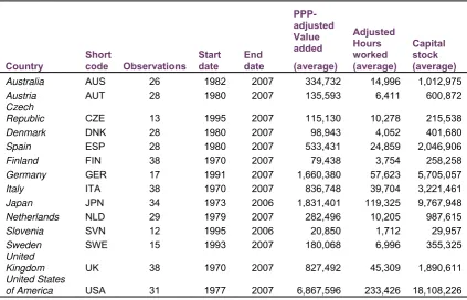
The countries that are included in the analysis together with the time periods for which data is available and the average values of the inputs and output are given in table 3.1 below. Overall, the productivity growth estimates are

produced for 14 different countries, over a number of years starting from 1970 and ending in 2007; on the whole the analysis includes 375 observations (each country in each time period as a different observation).

Table 3.1: Descriptive statistics of the dataset

Country

Short

code Observations Start date

End date

PPP-adjusted Value added (average)

Adjusted Hours worked (average)

Capital stock (average)

Australia AUS 26 1982 2007 334,732 14,996 1,012,975

Austria AUT 28 1980 2007 135,593 6,411 600,872

Czech

Republic CZE 13 1995 2007 115,130 10,278 215,538

Denmark DNK 28 1980 2007 98,943 4,052 401,680

Spain ESP 28 1980 2007 533,431 24,859 2,046,906

Finland FIN 38 1970 2007 79,438 3,754 258,258

Germany GER 17 1991 2007 1,660,380 57,623 5,705,057

Italy ITA 38 1970 2007 836,748 39,704 3,221,461

Japan JPN 34 1973 2006 1,831,401 119,325 9,767,948

Netherlands NLD 29 1979 2007 282,496 10,205 987,615

Slovenia SVN 12 1995 2006 20,850 1,712 29,957

Sweden SWE 15 1993 2007 180,068 6,996 355,325

United

Kingdom UK 38 1970 2007 827,492 45,309 1,890,611

United States

of America USA 31 1977 2007 6,867,596 233,426 18,108,226

3.2 Methodology

Productivity change is assessed in this study using the following approaches:

– GA (estimates are provided by the EU KLEMS project),

– DEA-based circular Malmquist indices,

– COLS-based Malmquist indices, and

– SFA-based Malmquist indices.

All frontier-based approaches examined in this analysis rely on the notion of what has come to be known as the Malmquist productivity index (Diewert, 1992), which has been used extensively in both the parametric (Kumbhakar & Lovell, 2000) and the non-parametric (Thanassoulis, 2001) setting.

Growth Accounting

Growth Accounting (GA) is an index number-based approach that relies on the neoclassical production framework, and seeks to estimate the rate of productivity change residually, ie by examining how much of an observed rate of change of a unit’s output can be explained by the rate of change of the combined inputs used in the production process. There are many

modifications that could be applied to the more general GA setting ((Balk, 2008); (del Gatto, et al., 2008)); however, most applications, including the EU KLEMS project, utilise ‘traditional’ growth accounting methods, as detailed in OECD (OECD, 2001) and briefly described here.

GA postulates the existence of a production technology that can be represented parametrically by a production function relating Value Added (YGVA), to primary inputs labour (L) and capital services (K) and productivity

change (TFP), which is Hicks-neutral, such that:

TFP L

K F

YGVA  ( , ) Eq. (2)

To parameterise (2), the analysis needs to adopt a number of assumptions, such as a constant returns to scale Cobb-Douglas production function and perfectly competitive markets; these are discussed in more detail in Annex 3 of the OECD manual (OECD, 2001).

If these assumptions hold, once the production function is differentiated with respect to time, the rate of change in output is equal to the sum of the

weighted average of the change in inputs and the change in productivity. The input weights are the output elasticities of each factor of production, which are derived as the share of each input to the total value of production. Therefore, productivity change is estimated by:

dt K d S dt

L d S dt

Y d dt

TFP

d K _i

i i L i GA

i

i

ln ln

ln

ln _{  }

Eq. (3)

where is the average share of labour in periods t and t-1, is the average share of capital in t and t-1 given by

L

i

S SiL

7_:

12

7

2 1 1 1 1             it it it L it it it it L it L Y p L w Y p L w

Si Eq.(4)

2 1 1 1 , 1 ,             it it it GA K it it it it GA K it K Y p K w Y p K w

Si Eq.(5)

It should be noted that the price of capital is not observable; as such, EU KLEMS, like the majority of GA applications (OECD, 2001), uses the so called endogenous ‘user cost of capital’ to estimate the final price of capital8_.

DEA-based Circular Malmquist index

The most common non-parametric approach for productivity measurement utilises Data Envelopment Analysis (DEA) to construct Malmqusit indices (MI) of productivity change. This approach was first proposed by Caves et al. (Caves, Christensen, & Diewert, 1982) and later refined by Färe et al. (Färe, Grosskopf, Norris, & Zhang, 1994).

This application utilises a circular Malmquist-type index (thereafter referred to as circular MI), which was first proposed by Pastor et al. (Pastor & Lovell, 2005) and refined by Portela et al. (Portela & Thanassoulis, 2010).

Whereas the ‘traditional’ MI uses two reference frontiers (based on the start and end period of the analysis) to compute the average distance between two points, the circular MI measures this distance using a single, common frontier as reference, which is constructed in such a way as to envelope all data points from all periods. This common frontier is defined as the ‘meta-frontier’ and since it allows for the full envelopment of the data across, it allows for the creation of a Malmquist-type index which is circular. Distances are measured by standard DEA models; for this application, we employ single output (PPP-adjusted real GVA), two input (Labour and Capital stock) constant returns to scale models.

The main advantages of the circular MI relative to the ‘traditional’ (Färe 1994) MI are the ease of computation and the ability to accommodate unbalanced panel data. For a more detailed discussion, see Portela et al. (Portela & Thanassoulis, 2010).

8

Corrected OLS

Corrected OLS (COLS) is a deterministic, parametric approach and one of the numerous ways that have been suggested to ‘correct’ the inconsistency of the OLS-derived constant term of the regression when technical inefficiency is present in the production process.

Two different COLS model specifications are used for this application. Both are based on a pooled regression model (ie all observations are included in the same model with no unit-specific effect). The first model assumes a Cobb-Douglas functional form and is given by:

it it

it

it L t

Y ln ln *

ln * *  *  Eq.(6) where *it are the estimated OLS residuals

The second COLS model specification assumes a translog functional form and is given by:

 





Inefficiency estimates are derived by:

Eq.(8) ) max( * * * it it it

u   



Productivity change is calculated by adding the different components of the Malmquist productivity index (see section Kumbhakar et al. (Kumbhakar & Lovell, 2000)) :

dt SEC d dt TC d dt EC d dt TFP

d itCOLS

COLS it COLS

it COLS

it / ln / ln / ln /

ln    Eq.(9)

where is the COLS-estimated efficiency change, is the COLS-estimated technical change and is the COLS-estimated scale

efficiency change.

COLS it

EC TC_itCOLS

COLS it SEC

Stochastic frontier analysis

The pre-eminent parametric frontier-based approach is Stochastic Frontier Analysis (SFA), which was developed independently by Aigner et al. (Aigner, Lovell, & Schmidt, 1977) and by Meeusen et al. (Meeusen & van den Broeck, 1977). The approach relies on the notion that the observed deviation from the

frontier could be due to both genuine inefficiency but also random effects, including measurement error. SFA attempts to disentangle those random effects by decomposing the residual of the parametric formulation of the production process into noise (random error) and inefficiency.

As is the case with the COLS approach, two separate SFA model

specifications are used in this application: one that adopts a Cobb-Douglas functional form and a second that adopts the translog. The models are very similar to those used under COLS; the only difference lies in the specification of the residual.

In more detail, the Cobb-Douglas model is given by:

it it it

it

it L t v u

Y  *ln  *ln  *  

ln    Eq.(10)

whereas the translog model is given by:

 





ln 2 2 2

         Eq.(11)

where represents the inefficiency component (and as such ) and represents measurement error ( ). The inefficiency component is estimated based on the JMLS (Jondrow, Knox Lovell, Materov, & Schmidt, 1982) estimator.

it

u u_it 0 vit

) , 0 ( ~ _v2

it N

v 

Two different distributions for the inefficiency component are tested:

– the exponential distribution, u_it ~Exp(_u) – the half-normal distribution, u_it ~N(0,_u2)

Productivity change is measured in exactly the same way as with COLS.

3.3 Results

16

Table 3.2: Annual TFP change estimates

TFP

measure DEA COLS

COLS translog

SFA (half-normal)

SFA

(exponential) SFA translog (half-normal)

SFA translog (exponential) GA Mean 0.52% 0.67% 0.86% 0.82% 0.82% 0.77% 0.88% 0.54% Std. Dev. 1.66% 1.44% 1.70% 1.14% 0.99% 1.69% 1.15% 1.44% Note: The parametric models that are not labelled as translog adopt the Cobb-Douglas functional form.

Table 3.2 shows that for the full period, TFP has been growing at an average annual rate of between 0.52% and 0.88%. The lowest average growth comes from the DEA-based circular Malmquist index, while the highest estimate comes from the translog SFA model that assumes an exponential distribution of inefficiency.

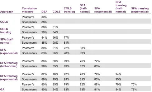
Table 3.3: Correlation coefficients for annual TFP change

Approach

Correlation

measure DEA COLS COLS translog

SFA (half-normal)

SFA

(exponential) SFA translog (half-normal)

SFA translog (exponential) Pearson's 89%

COLS Spearman's 88%

Pearson's 88% 81% COLS

translog Spearman's 90% 84%

Pearson's 84% 96% 77% SFA

(half-normal) Spearman's 85% 98% 81%

Pearson's 80% 91% 72% 98% SFA

(exponential) Spearman's 83% 96% 78% 99%

Pearson's 86% 80% 99% 76% 72% SFA translog

(half-normal) Spearman's 90% 85% 99% 82% 80%

Pearson's 82% 76% 92% 78% 79% 94% SFA translog

(exponential) Spearman's 86% 79% 93% 81% 80% 95%

Pearson's 80% 95% 79% 92% 88% 79% 75% GA Spearman's 80% 94% 83% 93% 91% 84% 78%

The overall similarity of the average TFP change estimates between the examined approaches is also apparent in the correlations between the estimates, presented in table 3.3 above. GA estimates are more highly correlated with the Cobb-Douglass COLS and SFA (half-normal) estimates and less highly correlated with the DEA and translog-specified parametric approaches. DEA estimates are more highly correlated with the COLS

that the translog SFA estimates are more highly correlated with each other and their translog COLS counterparts, while they display the smallest

correlation coefficients with the estimates from the Cobb-Douglas parametric models (COLS and SFA); this indicates that the selection of functional form to parameterise the models can have a large effect on the TFP growth

estimates, which was also observed in the simulation analysis undertaken in GET.

The results so far suggest that there appears to be a broad consensus between the various approaches. However average TFP change estimates across all countries masks the underlying variation observed at the

(individual) country level.

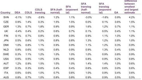
Table 3.4: Average annual TFP estimates by country

Country DEA COLS COLS translog

SFA (half-normal)

SFA (exponent ial)

SFA translog (half-normal)

SFA translog (exponent

ial) GA Difference between smallest and largest estimate SVN -0.1% 1.0% -2.6% 1.2% 1.1% -3.0% -1.6% 0.9% 4.2% CZE 0.9% 1.4% 0.3% 1.5% 1.5% 0.0% 0.1% 0.6% 1.5% GER 1.3% 0.7% 1.8% 0.9% 0.9% 1.6% 1.2% 0.7% 1.1% UK -0.4% 0.4% 0.2% 0.6% 0.7% 0.1% 0.5% 0.4% 1.1% FIN 0.1% 0.7% 0.8% 0.9% 0.9% 0.9% 1.1% 1.0% 1.0% JPN 0.5% 0.6% 1.5% 0.8% 0.8% 1.3% 1.2% 0.8% 1.0% DNK 1.0% 0.8% 1.1% 0.9% 0.9% 1.1% 1.2% 0.3% 0.9% NLD 0.8% 0.6% 1.0% 0.8% 0.9% 0.9% 1.3% 0.4% 0.9% SWE 0.3% 1.1% 1.2% 1.0% 1.0% 1.0% 0.9% 0.8% 0.9% USA 0.6% 0.5% 1.0% 0.9% 0.9% 0.8% 0.9% 0.2% 0.8% AUT 1.2% 0.9% 1.5% 1.0% 1.0% 1.4% 1.4% 1.0% 0.6% ESP 0.3% 0.3% 0.6% 0.4% 0.4% 0.6% 0.6% 0.0% 0.6% ITA 0.6% 0.6% 1.0% 0.7% 0.6% 1.0% 0.9% 0.4% 0.6% AUS 0.8% 0.7% 1.0% 0.8% 0.8% 0.9% 0.9% 0.5% 0.5%

Table 3.4 reveals that the various TFP change estimates at country level appear to be quite different, for some countries at least. This is despite the fact that correlations of the different estimates are still relatively high when comparing TFP growth estimates within an individual country9_{. On average,}

the difference between the smallest and the largest estimate is approximately

9

18

1.1 percentage points and for some countries this can be quite larger (eg the spread is 4.2 pc for SVN and 1.5 pc for CZE).

These, sometimes pronounced, differences in the TFP growth estimates between the different approaches can be problematic, if such analysis were to be used to inform policy. It is quite likely that a policy maker, upon presented such results would enquire as to why do the various estimates differ and, more importantly, which estimate is likely to be more accurate. The framework described in the next section aims to facilitate this selection process.

4

Applying the selection framework to the EU KLEMS

dataset

4.1 Assessing input volatility

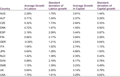
Input volatility is the easiest characteristic to assess; it is achieved by simply examining the annual change in inputs by country. Average input growth and its standard deviation is summarised in the table below.

Table 4.1: Average annual growth in inputs

Country

Average Growth in Labour

Standard deviation of Labour growth

Average Growth in Capital

Standard deviation of Capital growth AUS 2.29% 1.75% 3.81% 1.44% AUT 0.71% 1.24% 2.37% 0.29% CZE 0.32% 1.73% 2.84% 0.33% DNK 0.72% 1.57% 1.55% 0.92% ESP 2.19% 2.59% 3.44% 0.87%

FIN 0.84% 2.17% 3.94% 2.26%

GER -0.35% 1.21% 2.54% 0.64%

ITA 1.04% 1.02% 2.74% 1.13%

JPN 0.64% 1.28% 4.66% 1.93% NLD 1.42% 1.38% 2.35% 0.43% SVN 0.89% 2.18% 6.17% 0.76% SWE 1.15% 1.39% 3.23% 0.49%

UK 0.64% 2.20% 3.14% 0.79%

USA 1.70% 1.61% 3.29% 0.62%

relative volatility of labour input growth, measured as the ratio of standard deviation to average, is approximately 2.1 on average, while labour growth volatility in absolute terms, measured only by examining the standard deviation of the growth measure, is relatively small, averaging in approximately 1.7%.

Most countries have also been increasing their capital stock over the period of the analysis, with an average growth in capital inputs of 3.3%. Both relative and absolute volatility in capital input growth is quite low (compared with labour inputs), averaging at 0.3 and 0.9% respectively.

4.2 Assessing the extent of technical inefficiency

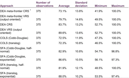
In order to provide an indication of how widespread technical inefficiency is in the countries in EU KLEMS dataset, this analysis examines the various estimates for the different approaches (and models) adopted; these are summarised in the following table.

Table 4.2: Average technical efficiency estimates, by approach

Approach

Number of

observations Average

Standard

deviation Minimum Maximum DEA meta-frontier CRS 1 375 73.1% 13.8% 41.9% 100.0% DEA meta-frontier VRS

(output oriented) 1 375 79.7% 14.6% 49.5% 100.0% DEA CRS 375 83.7% 13.2% 52.7% 100.0%

DEA VRS (output

oriented) 375 89.6% 13.6% 52.7% 100.0% COLS (Cobb-Douglas) 375 72.5% 11.9% 47.3% 100.0% COLS (translog) 375 72.3% 10.8% 46.5% 100.0% SFA (Cobb-Douglas,

half-normal) 375 82.9% 10.8% 54.7% 96.8% SFA (Cobb-Douglas,

exponential) 375 86.6% 10.5% 56.1% 97.3% SFA (translog,

half-normal) 375 81.9% 12.1% 48.5% 100.0% SFA (translog,

exponential) 375 88.0% 10.2% 53.5% 97.4% Note: 1 DEA meta-frontier efficiency estimates do not take into account the time dimension (technical change and scale efficiency change) and as such are likely to be biased (downward if we assume positive technical change). They are presented here for completeness.

20

Table 4.2 reveals a relative small spread of average efficiency in all the approaches examined. The two COLS specifications display the smallest average efficiency (approximately 72%), while the DEA output oriented VRS models display the largest average efficiency scores (approximately 90%). Average efficiency across all models is estimated at approximately 81% or 82% if the DEA meta-frontier efficiency scores are excluded (see note to table 4.2).

4.3 Assessing the extent of noise in the data

The relevant estimates of σv, the estimated standard deviation of the noise

component, from all the SFA models adopted for this application are provided in the table below.

Table 4.3: Summary statistics of the σv estimate from the SFA models

SFA model Estimate of σν

Standard deviation of the σν

estimate Minimum Maximum Cobb-Douglas,

half-normal 0.075 0.010 0.058 0.098

Cobb-Douglas,

exponential 0.086 0.007 0.073 0.101

Translog, half-normal 0.000 0.000 0.000 0.000 Translog, exponential 0.074 0.006 0.063 0.087

The two Cobb-Douglas models and the translog model that assumes technical inefficiency is exponentially distributed find that the standard

deviation of the normally-distributed error term is between 0.05 to 0.1. On the other hand, the translog SFA model that assumes half-normally distributed technical inefficiency finds that the amount of noise in the current dataset is negligible (σv is approximately equal to zero). This last finding appears quite

imputations10_{, it is expected that the data would almost always incorporate}

some degree of inaccuracy11_{. As such, it is unlikely that the EU KLEMS}

dataset is completely free of measurement error and/or statistical noise. Since the estimate of σv is inconsistent in the pooled setting, in order to

provide some clarity on whether the use of the σv estimate is valid in this

instance, it would be helpful to observe the behaviour of the estimate under controlled conditions through the use of simulation analysis.

This analysis utilises the same simulation framework12 _{presented in GET. The}

simulation experiment carried out in this instance utilises a DGP constructed in such a way that it displays similar characteristics as those observed in the EU KLEMS dataset. In more detail, the DGP:

– is a piece-wise linear production function, since the analysis in section 4.5 below suggests that the underlying production function in the current dataset is neither Cobb-Douglas nor translog13_;

– utilises input and price data that were constructed so that they are consistent with the level of input volatility observed in the EU KLEMS dataset (section 4.1). In summary, input quantities and price are randomly generated for the first period and then scaled by a random factor that follows N~(0.0.1);

– includes a technical inefficiency component, _(1/7) , which results in average technical efficiency levels in the simulations of appr. 88%. This is consistent with the estimates of technical inefficiency observed in the EU KLEMS dataset, as detailed in section 4.2 of this chapter;

~Exp u_it

– and lastly, includes a noise component that is randomly generated

following N~(0, 0.05), consistent with the estimates presented in table 4.3; The summary findings of the simulation analysis are given below:

10

See for example the requirement to incorporate imputed rents for owners/occupiers and the methodology used to estimate GVA from privately held corporations and unincorporated enterprises, as detailed in the ESA 1995 framework for National accounts.

11

This is also evident from the number of times that National Account information is updated, sometimes quite a few years after the original estimates were first published.

12

As a reminder, the simulation framework in question uses 100 observations (20 DMU observed over a 5 periods) and summarises the findings of 100 experiments.

13

22

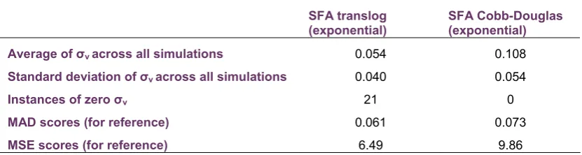
Table 4.4: Summary statistics of the σv estimate from the simulation analysis

SFA translog (exponential)

SFA Cobb-Douglas (exponential)

Average of σ_νacross all simulations 0.054 0.108 Standard deviation of σνacross all simulations 0.040 0.054

Instances of zero σν 21 0

MAD scores (for reference) 0.061 0.073

MSE scores (for reference) 6.49 9.86

The results show that the translog SFA model, which is the most accurate of the SFA models under these conditions with regards to productivity change estimates according to GET, displays an average estimate of σ_ν that is very close to its true value. However, the standard deviation of this average measure is quite large; the 95% upper confidence interval is approximately 0.135, which is more than twice as large as the true value. The simulation analysis also finds that out of the 100 simulation experiments, in 21 of those the translog SFA models displayed an estimated σνthat was approximately

equal to zero. This suggests that sometimes even the more accurate SFA model is not able to detect the presence of noise, even though modest levels of noise are part of the DGP. For the Cobb-Douglass SFA model, there were no instances where σνapproached zero, but the σν estimate was also twice as

large on average as the true standard deviation of the noise component. Overall, the results from the simulations demonstrate that in conditions that approximate those found in the current analysis, the estimate of σ_ν can provide an overall indication of the extend of measurement error/noise in the data, with the caveat that high levels of precision should not be expected.

4.4 Are the parametric models miss-specified?

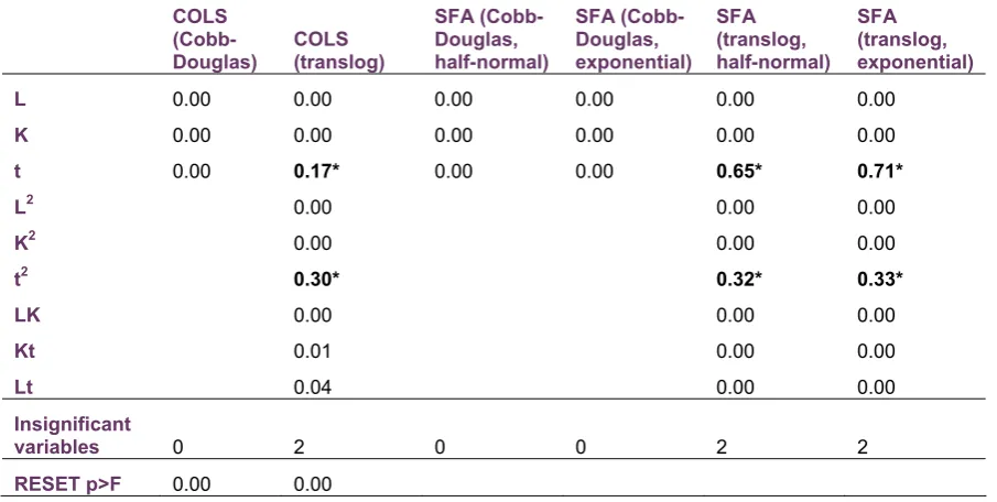
Table 4.5: Statistical significance of the variables in the parametric models and RESET test results from the application

COLS (Cobb-Douglas)

COLS (translog)

SFA (Cobb-Douglas, half-normal)

SFA (Cobb-Douglas, exponential)

SFA (translog, half-normal)

SFA (translog, exponential)

L 0.00 0.00 0.00 0.00 0.00 0.00

K 0.00 0.00 0.00 0.00 0.00 0.00

t 0.00 0.17* 0.00 0.00 0.65* 0.71*

L2 0.00 0.00 0.00

K2 0.00 0.00 0.00

t2 0.30* 0.32* 0.33*

LK 0.00 0.00 0.00

Kt 0.01 0.00 0.00

Lt 0.04 0.00 0.00

Insignificant

variables 0 2 0 0 2 2

RESET p>F 0.00 0.00

The analysis found that both the Cobb-Douglas and the translog models failed to pass the RESET test; in addition, all translog models found that the time variable and its square displayed coefficients that were statistically

insignificant. Both of these factors suggest that the parametric models could suffer from some form of miss-specification.

The next step is to test whether parametric models that are known to be miss-specified also display similar symptoms; this is achieved by a round of

24

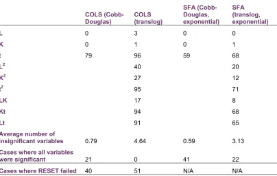
Table 4.6: Summary of statistical significance of the variables in the parametric models of the simulation analysis

COLS (Cobb-Douglas)

COLS (translog)

SFA (Cobb-Douglas, exponential)

SFA (translog, exponential)

L 0 3 0 0

K 0 1 0 1

t 79 96 59 68

L2 40 20

K2 27 12

t2 95 71

LK 17 8

Kt 94 68

Lt 91 65

Average number of

insignificant variables 0.79 4.64 0.59 3.13 Cases where all variables

were significant 21 0 41 22

Cases where RESET failed 40 51 N/A N/A

The simulation analysis shows that the RESET test found evidence of miss-specification in almost half of the simulation experiments. In addition, there were instances of insignificant variables in the majority of the experiments undertaken; the translog COLS specification had no cases where all variable were significant, while the Cobb-Douglas SFA model that (correctly) assumed exponentially-distributed inefficiency was the better performing model in this measure, with just 41 cases where all variables were statistically significant. Overall, these results suggest that when the parametric models suffer from functional form miss-specification, possible symptoms include statistical insignificant variables and failures in the RESET test. Given that similar symptoms where observed in the current application, one could conclude that the parametric models in this application are likely to suffer from some form of miss-specification, which would negatively impact the accuracy of their

productivity change estimates.

4.5 Selecting the most appropriate estimation approach

– input volatility is quite low, averaging just 1.7% p.a. for the labour input and 0.9% p.a. for the capital input (section 4.1);

– average technical inefficiency across all approaches in this application is approximately 82% (section 4.2);

– the SFA models suggest that the standard deviation of the normally-distributed noise component (σν) probably takes a value between 0.05

and 0.1 (section 4.3);

– the parametric models are likely to suffer from some form of

miss-specification, which could be due to the adopted functional form not being an appropriate representation of the underlying DGP section 4.4);

According to the above findings, the simulation experiment from GET that more closely matches the characteristics of the current dataset is S2.3 with ‘default’ input volatility. In more detail, for the S2.3 simulation experiment:

– the underlying DGP is piecewise-linear, since the current analysis found that neither the Cobb-Douglas nor the more flexible translog functional forms provide a close approximation to the underlying DGP.

– inputs are scaled from one year to the next by a random factors that follows N~(0,0.1), which results in input volatility similar the EU KLEMS dataset.

– average technical efficiency in the simulations is designed to be

approximately 87% on average - the current analysis found that average technical efficiency across all approaches in the EU KLEMS dataset is 82%.

– includes a noise component in the DGP, which is randomly generated and follows N~(0,0.05). The decision to adopt this level of noise could be considered conservative, since the mid-point between the various chosen estimates of σν is closer to 0.075.

26

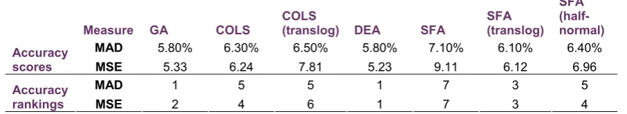
Table 4.7: Summary accuracy results

Measure GA COLS

COLS

(translog) DEA SFA SFA (translog)

SFA (half-normal)

MAD 5.80% 6.30% 6.50% 5.80% 7.10% 6.10% 6.40% Accuracy

scores MSE 5.33 6.24 7.81 5.23 9.11 6.12 6.96

MAD 1 5 5 1 7 3 5

Accuracy

rankings MSE 2 4 6 1 7 3 4

Note: MAD = Mean Absolute deviation, MSE = Mean Square Error

As table 4.7 demonstrates, the two most accurate approaches in this simulation experiment were DEA and GA, closely followed by the translog SFA model. The DEA and GA accuracy scores are almost identical; it should be noted however that the simulation analysis is designed such that the relevant input and output prices indices required by GA are measured with no error, while also explicitly assuming that there is no element of allocative inefficiency in the analysis. The reason for designing the experiment in such a way was that it allowed for a level playing field when comparing the GA with the frontier-based estimates, which do not rely on price information. In a real life application such as the current analysis however, some amount of

measurement error is expected to be present in the price data; in addition, the GA estimates would also be influenced by changes in allocative inefficiency in the countries examined. Given that the impact of those factors to the relative accuracy of the GA estimates under the current conditions is unknown, it would be more prudent to rely mostly on the DEA-based productivity estimates.

5

Summary and conclusions

The aim of this paper was to devise a selection framework to help policy makers choose the productivity measurement approach that is likely to produce the most accurate estimates relative to the application in hand. This selection framework includes three steps:

– First, determine those conditions/characteristics inherent in the DGP that can have a significant influence in the relative accuracy of the assessed productivity measurement approaches.

– Finally, examine the relative accuracy of the adopted approaches in datasets specifically designed to display those characteristics/factors found the real-life data of the current application.

With regards to the fist step, we rely on the findings of the simulation analysis undertaken in GET, which identified that the characteristics of the DGP that are most influential the overall accuracy of the most common productivity measurement approaches include: input volatility, technical inefficiency, noise and whether the parametric approaches are likely to suffer from functional form misspecification. The above list is not necessarily exhaustive and here may well be additional characteristics that have a significant impact on the overall accuracy of productivity change estimates, such as latent

heterogeneity amongst the assessed units and variable returns to scale. We leave the assessment of these and other potentially significant characteristics for future research.

At the second step, we attempt to assess whether and to what extent the above characteristics are present in the application at hand. To do so we propose the use of a number of well-established diagnostics and indicators so that the proposed selection framework can be easily implementable, such as RESET for assessing functional form miss-specification and estimates of technical efficiency derived from the assessed approaches. As was mentioned before, the results of such analysis should not be taken as absolutes, especially regarding the noise estimates and the presence of functional form miss-specification. Nevertheless, the simulation analysis undertaken in this paper does demonstrate that such can provide relatively reliable estimates. Hopefully, more focused diagnostics/indicators can be developed and refined in the future.

28

As an example of how this selection framework can be implemented in

practice, we assess the productivity performance of a number of EU countries using the EU KLEMS dataset. The analysis found that although at first glance all assessed approaches (namely Growth Accounting, Circular DEA-based Malmquist indices and COLS- and SFA-based Malmquist indices) produce very similar productivity change estimates on average, the productivity estimates from the various approaches are quite dissimilar at the individual country level. These differences are problematic from a policy perspective, since policy decisions on the issue of economic growth rely on having

accurate productivity estimates at the national level. By applying the proposed selection framework, it was possible to derive that the approach that is likely to provide the most accurate estimates in this instance was the DEA-based Malmquist indices. We propose that such a selection framework (hopefully refined and expanded in future iterations) can help improve our understanding of the complex issue of productivity change.

References

Aigner, D., Lovell, C. A. K., & Schmidt, P. (1977). Formulation and estimation of

stochastic frontier production function models. Journal of Econometrics, 6,

21-37.

Balk, B. (2008). Measuring Productivity Change Without Neoclassical Assumptions:

A Conceptual Analysis. In ERIM Report Series Reference No.

ERS-2008-077-MKT.

Banker, R. D., Chang, H., & Cooper, W. W. (2004). A simulation study of DEA and

parametric frontier models in the presence of heteroscedasticity. European

Journal of Operational Research, 153, 624-640.

Caves, D. W., Christensen, L. R., & Diewert, W. E. (1982). The Economic Theory of

Index Numbers and the Measurement of Input, Output, and Productivity.

Econometrica, 50, 1393-1414.

Coelli, T. (2002). A comparison of alternative productivity growth measures: with

application to electricity generation. In K. J. Fox (Ed.), Efficiency in the Public

Sector: Springer.

del Gatto, M., di Liberto, A., & Petraglia, C. (2008). Measuring Productivity. In: Centre

for North South Economic Research, University of Cagliari and Sassari,

Sardinia.

Diewert, W. E. (1992). The Measurement of Productivity. Bulletin of Economic

EU KLEMS. (2008). EU KLEMS Database, see Marcel Timmer, Mary O'Mahony &

Bart van Ark, The EU KLEMS Growth and Productivity Accounts: An

Overview, University of Groningen & University of Birmingham. In.

Eurostat, & OECD. (2007). Methodological Manual on Purchasing Power Parities. In:

European Commission.

Färe, R., Grosskopf, S., Norris, M., & Zhang, Z. (1994). Productivity Growth,

Technical Progress, and Efficiency Change in Industrialized Countries.

American Economic Review, 84, 66-83.

Fried, H. O., Lovell, C. A. K., & Schmidt, S. S. (2008). The Measurement of

Productive Efficiency and Productivity Growth. In: Oxford University Press.

Jacobs, R. (2001). Alternative Methods to Examine Hospital Efficiency: Data

Envelopment Analysis and Stochastic Frontier Analysis. Health Care

Management Science, 4, 103-115.

Jondrow, J., Knox Lovell, C. A., Materov, I. S., & Schmidt, P. (1982). On the

estimation of technical inefficiency in the stochastic frontier production

function model. Journal of Econometrics, 19, 233-238.

Knox Lovell, C. A. (1996). Applying efficiency measurement techniques to the

measurement of productivity change. Journal of Productivity Analysis, 7,

329-340.

Kumbhakar, S. C., & Lovell, C. A. K. (2000). Stochastic Frontier Analysis: Cambridge

University Press.

Meeusen, W., & van den Broeck, J. (1977). Efficiency Estimation from Cobb-Douglas

Production Functions with Composed Error. International Economic Review,

18, 435-444.

Odeck, J. (2007). Measuring technical efficiency and productivity growth: a

comparison of SFA and DEA on Norwegian grain production data. Applied

Economics, 39, 2617-2630.

OECD. (2001). Measuring Productivity: Measurement of Aggregate and

Industry-Level Productivity Growth. In: OECD.

OECD. (2009). Measuring Capital. In.

Pastor, J. T., & Lovell, C. A. K. (2005). A global Malmquist productivity index.

Economics Letters, 88, 266-271.

Portela, M. C. A. S., & Thanassoulis, E. (2010). Malmquist-type indices in the

presence of negative data: An application to bank branches. Journal of

Banking & Finance, 34, 1472-1483.

Resti, A. (2000). Efficiency measurement for multi-product industries: A comparison

of classic and recent techniques based on simulated data. European Journal

30 Solow, R. M. (1957). Technical Change and the Aggregate Production Function. The

Review of Economics and Statistics, 39, 312-320.

Thanassoulis, E. (2001). Introduction to the Theory and Application of Data