Use of satellite derived data for characterization of snow cover and simulation of snowmelt runoff through a distributed physically based model of runoff generation

www.hydrol-earth-syst-sci.net/14/339/2010/ © Author(s) 2010. This work is distributed under the Creative Commons Attribution 3.0 License.

Hydrology and

Earth System

Sciences

Use of satellite-derived data for characterization of snow cover and

simulation of snowmelt runoff through a distributed physically

based model of runoff generation

L. S. Kuchment1, P. Romanov2, A. N. Gelfan1, and V. N. Demidov1

1_{Water Problem Institute of the Russian Academy of Sciences, Moscow, Russia} 2_{University of Maryland, College Park, MD, USA}

Received: 22 July 2009 – Published in Hydrol. Earth Syst. Sci. Discuss.: 12 August 2009 Revised: 29 January 2010 – Accepted: 1 February 2010 – Published: 22 February 2010

Abstract. A technique of using satellite-derived data for

constructing continuous snow characteristics fields for dis-tributed snowmelt runoff simulation is presented. The satellite-derived data and the available ground-based mete-orological measurements are incorporated in a physically based snowpack model. The snowpack model describes tem-poral changes of the snow depth, density and water equiva-lent (SWE), accounting for snow melt, sublimation, refreez-ing melt water and snow metamorphism processes with a special focus on forest cover effects. The remote sensing data used in the model consist of products include the daily maps of snow covered area (SCA) and SWE derived from obser-vations of MODIS and AMSR-E instruments onboard Terra and Aqua satellites as well as available maps of land sur-face temperature, sursur-face albedo, land cover classes and tree cover fraction. The model was first calibrated against avail-able ground-based snow measurements and then applied to calculate the spatial distribution of snow characteristics using satellite data and interpolated ground-based meteorological data. The satellite-derived SWE data were used for assigning initial conditions and the SCA data were used for control of snow cover simulation. The simulated spatial distributions of snow characteristics were incorporated in a distributed physi-cally based model of runoff generation to calculate snowmelt runoff hydrographs. The presented technique was applied to a study area of approximately 200 000 km2including the Vy-atka River basin with catchment area of 124 000 km2. The

Correspondence to: A. Gelfan ([email protected])

correspondence of simulated and observed hydrographs in the Vyatka River are considered as an indicator of the ac-curacy of constructed fields of snow characteristics and as a measure of effectiveness of utilizing satellite-derived SWE data for runoff simulation.

1 Introduction

2002). However, the potential of satellite snow data is lim-ited by a number of environmental factors (cloudiness, land cover type, terrain peculiarities, etc.) as well as by insuf-ficient, in many cases, accuracy of satellite measurements. Clouds create discontinuity in the spatial distribution and in time series of snow data. Dense forest vegetation compli-cates snow cover identification and mapping due to snow in-terception and ability to mask snow cover on the forest floor. The accuracy of satellite measurements of snow water equiv-alent (SWA) significantly depends on the actual properties of the snow, especially the amount of liquid water.

A possible way to improve characterization of the snow spatial distribution and temporal variability consists in cou-pling satellite snow cover products with ground-based mete-orological measurements and snow pack models. Most of the studies are focused at using satellite measurements of snow covered area (SCA) (e.g. Rodell and Houser, 2004, An-dreadis and Lettenmaier, 2006, Dressler et al., 2006, Kolberg et al., 2006). US National Operational Hydrologic Remote Sensing Center (NOHRSC) has developed a Snow Data As-similating System (SNODAS) where the ground-based, air-borne and satellite snow observations were assimilated into the snow model to obtain the snow cover characteristics at 1 km spatial resolution and hourly temporal resolution (Car-roll et al., 2006). A joint US Air Force/NASA blended, global snow product named “ANSA” utilizing both MODIS, AMSR-E and QuikSCAT sensor data has been developed and presented in (Foster et al., 2007).

In this paper we present a technique for constructing space-time continuous fields of snow cover characteristics (SWE, snow depth, snowmelt, etc.) on the basis of a physi-cally based model of snow pack and with the use of satellite measurements of SWE. Satellite SCA products are used for control of the calculated snow cover fields and for calibra-tion of the snow model. Satellite products also include maps of land surface temperature and albedo, which are utilized by the model when these maps are available. The model is first calibrated against available snow measurements at meteorological stations. Next, satellite-derived SWE maps specifically corrected for forested areas are utilized as the initial conditions and ground-based meteorological data as boundary conditions to simulate the spatial distribution of snow characteristics. Finally, the simulated spatial distribu-tions of snow cover characteristics are incorporated in a dis-tributed physically based model of runoff generation to cal-culate snowmelt runoff hydrographs. The correspondence of simulated and observed hydrographs may be considered as an indicator of the accuracy of the constructed fields of snow characteristics and at the same time, as a measure of effec-tiveness of utilizing satellite-derived SWE data as the initial conditions for runoff simulation. It is obvious a priory that because of possible large errors in satellite SWE maps such utilizing can be effective if the ground-based meteorologi-cal network is sparse and does not represent properly spatial heterogeneities of snow characteristics.

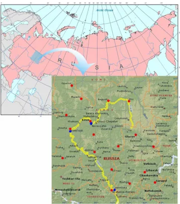
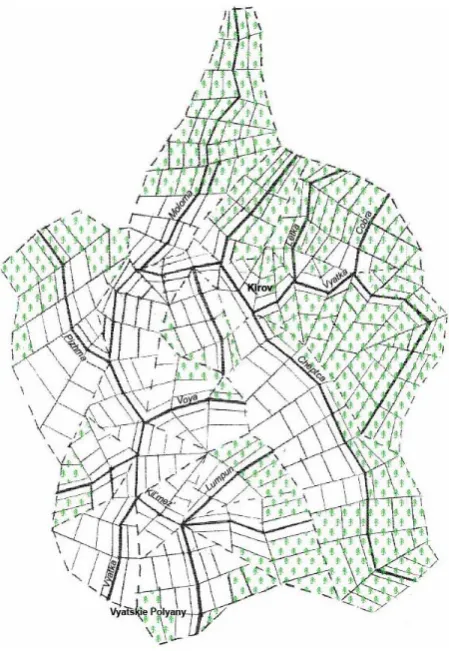
The current technique was applied to a study area of about 200 000 km2 located in the European part of Russia with 56◦_N–60◦_{N and 48}◦_E–54◦_{E spatial coordinates. The study}

area incorporates the Vyatka River basin with a catchment area of approximately 124 000 km2 (Fig. 1), for which this technique was used for simulation of snowmelt runoff hy-drographs.

The study area has flat terrain and mixed vegetation cover. In its northern part more than 80% of the area is covered by coniferous and mixed forests. The southern part is mostly agricultural land with less than 10–15% forest cover (Fig. 2). The snow season lasts for about 5 months with seldom thaws. Maximum snow water equivalent accumulates in the end of March and ranges from 100–120 mm in the south of the re-gion to about 200–250 mm in the north. Snow melting starts, on average, on the 27 March and ends in the beginning of May.

2 Satellite and ground-based information used in

the study

On the basis of measurements from the Advanced Mi-crowave Scanning Radiometer (AMSR-E) of NASA’s Earth Observing System (EOS) Aqua satellite, NASA issues since 2002 daily maps of SWE for the entire globe with 0.2◦ grid pixel size of the latitude-longitude projection (AMSR-E/Aqua Daily L3 Global Snow Water Equivalent EASE-Grids – AE-DySno). These maps are computed using the empirical relationship between SWE and the difference in brightness temperature of the land surface at 18 and 36 GHz using appropriate fractions of forest cover and assuming ver-tical polarization. The potential error in SWE estimates us-ing this satellite and retrieval algorithm is about 25% (Chang and Rango, 2000), yet for forested areas these errors can be significantly larger. Moreover, the accuracy of the SWE es-timated from the radiometric satellite measurements notice-ably decreases during melt period when snowpack is satu-rated by melted water (Engen et al., 2004). Significant errors can occur during thawing and when the land surface contains a thin ice crust. In addition, study by Dong et al. (2005) shows that the SWE retrievals are not sensitive to thin snow packs (SWE<10 mm). Results of validation of daily maps AE-DySno against ground snow courses for several test areas in the European part of Russia have shown that the satellite-derived values of SWE before snowmelt can deviate as much as 200% from the actual ground SWE values (Nosenko et al., 2006).

1

2

3

Fig. 1. Location of the study region (red points – meteorological gauges; blue points – hydrological

gauges). The Vyatka River is highlighted in yellow.

Fig. 1. Location of the study region (red points – meteorological gauges; blue points – hydrological gauges). The Vyatka River is highlighted in yellow.

enough daylight to be properly classified or did not pass any of data quality control tests. Earlier estimates of the accu-racy of MODIS-based snow cover maps range from 90% to 98% depending on the season and the surface type (Hall and Riggs, 2007). Most studies report a substantial increase in snow detection error in forested areas (e.g. Simic et al., 2004).

The satellite information used in this study includes AE-DySno and MOD10 L2 maps as well as be-daily land surface temperature maps MOD11 L2 and albedo maps of albedo MOD43C1 derived at 5 km resolution from MODIS-Terra re-flective channels data accumulated over 16-day periods. The accuracy of land surface temperature estimates is close to 1◦C.

Besides current MODIS and AMSR-E data, we also used static datasets such as type of land surface and the type and density of forest vegetation cover. All latter data products are

based on observations from AVHRR aboard NOAA’s satel-lite (Hansen et al., 2000). They have been produced at the University of Maryland Department of Geography and were acquired from http://glcf.umiacs.umd.edu/data.

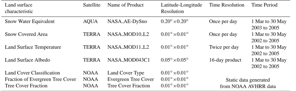
The full list of the satellite products used in the present work is given in Table 1. Figure 3 shows examples of SWE, SCA, surface temperature and albedo maps. As can be seen from these maps, the satellite data reveal significant spatial heterogeneity of the considered variables.

Table 1. List of satellite data products used in the study.

Land surface Satellite Name of Product Latitude-Longitude Time Resolution Time Period

characteristic Resolution

Snow Water Equivalent AQUA NASA AE-DySno 0.20◦×0.20◦ Once per day 1 Mar to 30 May

2003 to 2005

Snow Covered Area TERRA NASA MOD10 L2 0.01◦×0.01◦ Once per day 1 Mar to 30 May

2002 to 2005

Land Surface Temperature TERRA NASA MOD11 L2 0.01◦×0.01◦ Twice per day 1 Mar to 30 May

2002 to 2005

Land Surface Albedo TERRA NASA MOD043C1 0.05◦×0.05◦ 16-day product 1 Mar to 30 May

2002 to 2005

Land Cover Classification NOAA Land Cover Type 0.01◦×0.01◦

Static data generated

Fraction of Evergreen Tree Cover NOAA Evergreen Tree Cover 0.01◦×0.01◦

from NOAA AVHRR data

Tree Cover Fraction NOAA Tree Cover Fraction 0.01◦×0.01◦

1 2 3 4

Fig. 2. Land cover classification within the study region

Fig. 2. Land cover classification within the study region.

3 Snow pack model, its calibration and validation using

ground-based data

The snow pack model (Gelfan et al., 2004; Kuchment and Gelfan, 2004) used in this study is a system of vertically averaged equations which includes description of temporal changes of the snow depth, contents of ice and liquid water taking into account snow melt, sublimation, refreezing melt water, and snow metamorphism:

dH

dt =ρw

h

Xsρ0−1−(S+Es)(ρii)−1

i

−V (1)

d

dt(iH )=

ρw

ρi

(Xs−S−Es)+Si (2)

d

dt(wH )=Xl+S−El−R−

ρi

ρw

Si (3)

cs

d

dt(TsH )=Qa−Qg−ρwLS+ρiLSi (4)

whereH represents the snow depth;iandwsignify the vol-umetric content of ice and liquid water, respectively;Ts

de-notes the temperature of snowpack; S represents the snow melt rate;Si signifies the rate of freezing of liquid water in

snow,El denotes the rate of liquid water evaporation from

snow; Es represents the rate of snow sublimation, Qa

sig-nifies the net heat flux at the snow surface;Qg denotes the

ground heat flux;Xs andXlrepresent the snowfall and

rain-fall rate at the snow surface, respectively; V signifies the snowpack compression rate;Rdenotes the snowmelt outflow from snowpack; cs represents the specific heat capacity of

snow;ρw,ρi, andρ0signify the densities of water, ice, and fresh-fallen snow, respectively;Ldenotes the latent heat of ice fusion.

The snow melt rate,S, is computed from the energy bal-ance of the snowpack atTs=0◦C as:

S=

Qa−Qg

(ρwL)−1=Qsw+Qlw−Qls+QT+QE+QP−Qg

(ρwL)−1,Qa−Qg>0

0,Qa−Qg<0

(5) whereQswrepresents the net short wave radiation;Qlw sig-nifies the downward long wave radiation;Qlsdenotes the up-ward long wave radiation from snow;QT represents the

sen-sible heat exchange;QE signifies the latent heat exchange;

QP denotes the heat content of liquid precipitation.

Radiation fluxes are calculated differently depending on the properties of the vegetation cover. Components of Qa

(in W m−2)for an open site are calculated as follows. The net short wave radiation and long wave radiation are ex-pressed with the empirical relationships (Eqs. 6–9) where the observed air temperature, air humidity, wind speed, precipi-tation, and cloudiness are used as input:

1

2

3

4

Fig. 3 The satellite-derived maps of SWE, SCA, land surface temperature and albedo for the study

area

Fig. 3. The satellite-derived maps of SWE, SCA, land surface temperature and albedo for the study area.

whereQ0=1000β represents the short-wave radiation flux under clear sky conditions for the day and the hour in ques-tion;β denotes the angle of short-wave radiation above the horizontal in radians, calculated as a function of the local lat-itude, the declination, and the hour angle; andαssignifies the

snow albedo calculated from:

αs=α0−ρsρw−1 (7)

in whichα0 represents an empirical coefficient; ρs denotes

the density of snowpack equalρs=ρii+ρww; N andN0 signify the total and the lower level cloudiness (ratiometric), respectively;

Qlw=σ Ta4

0.61+0.05e0_a.5(1.00+0.12N+0.12N0) (8)

Qls=εsσ Ts4 (9)

where σ represents the Stefan-Boltzmann constant (W m−2K−4); ea denotes the air vapor pressure (mb),

εs signifies the effective emissivity of the snowpack taken

equal to 0.99 in this study

The turbulent fluxes of sensible and latent heat are calcu-lated using:

QT=

_ρ

aca

ra

+qT

(Ta−Ts) (10)

QE=

₀

.622Lsρa

Para

+qE

(ea−es) (11)

wherera represents the aerodynamic resistance;es denotes

the saturation air vapor pressure at the temperature of snow surface; ρ0signifies the air density;ca denotes the specific

heat capacity of air;Parepresents the atmospheric pressure;

Ls signifies the latent heat of sublimation of ice in the

ab-sence of liquid water or the latent heat of vaporisation when liquid water is present in snow; qT and qE represent the

wind-less convection coefficients for the sensible and the la-tent heat fluxes, respectively. The coefficients qT andqE

The aerodynamic resistance is calculated as follows:

ra=

h lnz−_zH

0 i2

κ2_U

z

×(1+10|Ri|), (12)

whereUzrepresents wind speed at the heightz; z0denotes the snow surface roughness assigned as 0.005 m; κ repre-sents von Karman’s constant, and Ri is the Richardson num-ber whose value is estimated using:

Ri=g(Ta−Ts)(z−H ) U2

z[0.5(Ta+Ts)]

, (13)

wheregis the acceleration due to gravity.

The heat fluxQP caused by the liquid precipitation is

ex-pressed as:

QP =ρwcwTaXl (14)

wherecwrepresents the specific heat capacity of water.

The ground heat fluxQgis found from Eq. (28) describing

the vertical heat transfer in soil.

At the forest floor, Eqs. (8) and (9) are modified to take into account the effect of canopy coverage and the type of vegeta-tion on radiavegeta-tion fluxes. Net short wave radiavegeta-tion (Q∗_sw)and downward long wave radiation (Q∗_lw)fluxes on sub-canopy snow surface are calculated as:

Q∗_sw=Qsw(1−Cc+kswCc) (15)

Q∗_lw=CcQlc+(1−Cc)Qlw (16)

whereCc represents the canopy coverage (ratiometric);ksw denotes the transmissivity through the canopy;Qlcspecifies the long-wave radiation emitted by the canopy (upward and downward), calculated as εcσ Tc4, where Tc represents the

temperature of canopy (◦K) and assumed equal to air tem-perature; εc denotes the emissivity of the canopy taken as

0.96.

Transmissivity is calculated using:

ksw=exp

−QextLAIsin−1β

(17) where LAI denotes the leaf area index;Qextrepresents the extinction efficiency estimated as: Qext=1.08βcosβ (β is in radians).

When calculating the turbulent heat exchange under forest canopy, it was assumed that air temperature and air humidity in forest are the same in the forest and in the open area ad-joining to the forest. The wind speed in forestU_z∗is defined as:

U_z∗=kuUz (18)

wherekudenotes the coefficient of wind shield calculated as:

ku=0.56exp(−2.25Cc), 0.2< Cc<0.9 (19)

It was assumed that the precipitation type changes from liq-uid to solid at an air temperature of 0◦C. Depending on the

snowfall rate and the forest type part of the snowfall may be intercepted by the forest canopy. For a single snowfall onto a snow-free canopy, the amount of snow intercepted by the forest canopy is defined as:

I=Imax

1−exp−X

∗

s

Imax

(20) where X_s∗ represents the snowfall rate above the canopy;

Imax=SpLAI

0.27+46ρ₀−1 represents the interception capacity, found as a function of the species snow loading co-efficient,Sp. The density of fresh-fallen snowρ0(in kg m−3) depends on the air temperature.

The rate of sublimation of intercepted snowEi is derived from the energy balance of the intercepted snow as:

Ei= −R_neti +Qi_T+QP

(ρwL)−1 (21)

whereR_neti represents the net radiation absorbed by the inter-cepted snow;Qi_T denotes the sensible heat exchange for the intercepted snow.

The net radiation,Ri_net, absorbed by the intercepted snow is expressed as:

R_neti =Qsw[1−αc−ksw(1−αs)]+Qlw+Qls−2Qlc (22) whereαcrepresents the canopy albedo taken equal to 0.12 in

this study.

The componentQi_T is calculated from the ice bulb tem-perature and wind speed (Gelfan et al., 2004).

The rate of liquid water freezing in snowpackSi is

calcu-lated as:

Si=

    

   

Hdw_dt,Ts=0◦C∧Qa−Qg<0∧

|Qa−Qg|

ρiL ≥H

dw dt

|Qa−Qg|

ρiL ,Ts=0

◦_C∧Q

a−Qg<0∧

|Qa−Qg|

ρiL < H

dw dt

0,Ts=0◦C∧Qa−Qg≥0

Xl,Ts<0◦C

(23)

The snowpack compression rateV is found from (in cm s−1):

V= v1ρs

exp(v2Ts+v3ρs)

H2

2 (24)

where the density of snowpack, ρs, is in g cm−3; v1, v2, andv3specify the coefficients equal 2.8×10−6cm2s−1g−1;

−0.08◦C−1; 21 cm3g−1, respectively.

The outflow of liquid water from snow is calculated as:

R=

Xl+S−El−wmaxdH_dt ,w=wmax 0,w < wmax

(25) wherewmaxrepresents the holding capacity of snowpack re-lated to its densityρs as:

wmax=0.11−0.11

ρw

ρs

simulation results. It was shown that decreasing of time step smaller than 6 h does not lead to increasing of simulation ac-curacy. As a result, time step of integration was 6 h, i.e. the same as the time-step of the input meteorological data.

The snow pack model was calibrated and validated using available measurements of snow depth at 19 meteorological stations. To calibrate the model we used snow depth data obtained during the time period from 1 November 2001 to 30 May 2002. The values ofα0 (Eq. 7), qT (Eq. 10) and

qE (Eq. 11) were calibrated against snow depth and found

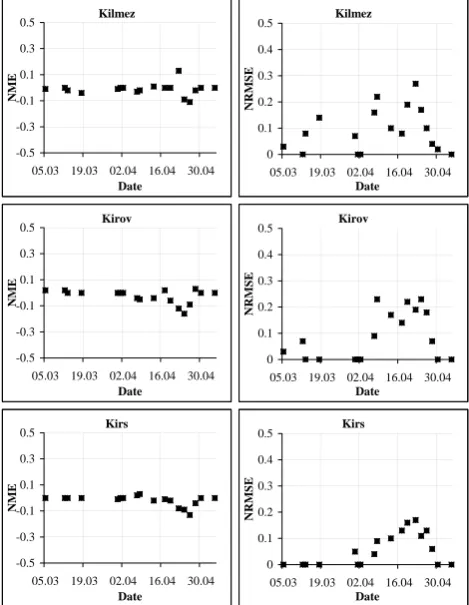
equal to 1.01, 0.98 J m−2s−1 and 0.11 J Pa−1s−1, respec-tively. Monte Carlo simulation was used to randomly gen-erate one hundred parameter sets, from which optimal pa-rameter set was identified. The papa-rameters were assumed to be uniformly distributed within the pre-determined intervals. The snow depth measurements at the same meteorological stations during the time period from 1 November 2002 to 30 May 2005 were used to assess the model performance. The standard deviations of differences (errors) between cal-culated and observed snow depths were estimated for each of 19 meteorological stations. The overall mean standard devia-tion of errors was equal to 7 cm for the calibradevia-tion period and increased to 9 cm for the validation period. As an illustration of the obtained results, Fig. 4 compares the results of snow depth simulations at several meteorological stations for the period of 1 November 2002 to 30 May 2003.

In order to test the validity of the model calibrated against the snow depth measurements in predicting SWE, we used the snow survey observations within the Vyatka River basin for 9 snow seasons: from 1971–1972 to 1979–1980. Both snow depth and SWE observations are available for that pe-riod. The model demonstrated satisfactory accuracy in pre-dicting SWE: the overall mean error is 1.2 mm with mean standard deviation of about 10.6 mm.

4 Modeling spatial fields of snow characteristics

The calibrated and validated snow pack model was applied to simulate the spatial distribution of snow pack characteristics over the study area during the time period from 1 March, when the SWE is typically close to the maximum value and errors of its satellite measurements have to be minimal, to 30 June of 2003–2005. The model was run for each 0.01◦ grid cell within the study area. To obtain the input data for the snow pack model, the daily ground-based meteorological observation data were interpolated to each pixel using the inverse distance squared method.

In the grid cells where the MODIS-based surface tem-perature and albedo data were not available, we calcu-lated surface temperature and albedo using Eqs. (4) and (7), respectively.

The initial spatial distribution of SWE for the open, i.e. forest-free, areas was assigned using AE-DySno SWE maps on 1 March. The SWE values for all forested pixels as well

Kilmez (56°56'N; 51°04'E)

0 10 20 30 40 50 60 70 80 90 100

01.09 10.12 20.03 28.06 06.10

Sno

w dept

h, cm

Kirov (58°36'N; 49°38'E)

0 20 40 60 80 100

01.09 10.12 20.03 28.06 06.10

Sno

w

dept

h,

cm

Kirs (59°21'N; 52°20'E)

0 20 40 60 80 100

01.09 10.12 20.03 28.06 06.10

Sno

w dept

h, cm

Kotelnich (58°18'N; 48°18'E)

0 20 40 60 80 100

01.09 10.12 20.03 28.06 06.10

Sno

w

dept

h,

cm

Kumeny (58°07'N; 49°53'E)

0 20 40 60 80 100

01.09 10.12 20.03 28.06 06.10

Sno w d ept h, cm

Lalsk (60°41'N; 47°36'E)

0 20 40 60 80 100

01.09 10.12 20.03 28.06 06.10

Sno

w

dept

h,

cm

Mozhga (56°26'N; 52°12'E)

0 20 40 60 80 100

01.09 10.12 20.03 28.06 06.10

S n o w depth, cm

Nagornoe (59°19'N; 50°50'E)

0 20 40 60 80 100

01.09 10.12 20.03 28.06 06.10

S n o w depth, cm 1 2 3

Fig. 4. Seasonal change of the observed (points) and simulated (line) snow depths (in cm) at selected stations within the study area for the season from November 2002 to June 2003

Fig. 4. Seasonal change of the observed (points) and simulated (line) snow depths (in cm) at selected stations within the study area for the season from November 2002 to June 2003.

as the missed SWE values for open pixels were estimated by interpolation from open pixels where satellite-derived SWE values were available. The interpolated SWE was further multiplied by the factorksnow, representing the average ra-tio of the pre-melt SWE in the forest to the pre-melt SWE in the neighboring open area. The value ofksnowwas obtained from numerical simulation of snow accumulation in the for-est with the snow cover model driven by meteorological ob-servations during 14 snow seasons from 1970–1971 to 1979– 1980 and from 2000–2001 to 2003–2004. The simulation results have shown that in the deciduous forest the value of

is 6–13% less to open ones. The numerical simulations have shown that the variations of the value ofksnowfrom year to year for the same forest area are small and can be negligible. Assuming that the spatial variability of snow density is much less than variability of SWE, the initial snow density on 1 March was accepted as constant for the whole area and defined from the measurements at the Kirov meteorological station. The initial volumetric moisture content of snow was assumed equal to zero.

Using the assumptions formulated above, we simu-lated daily maps of SCA and compared them with NASA MOD10 L2 SCA maps for the snowmelt season of the years 2002 and 2004. The comparison was carried out in or-der to refine the snow model parameters adjusted against the ground-based point measurements (see previous section) and use the refined parameters for further characterization of snow fields. The region was divided on to 19 Thissen poly-gons according to the location of the meteorological stations. Simulated, SCAcalc, and satellite-derived, SCAsat, values were estimated for each polygon and for the dates when most of the polygons were free of cloudiness. The value of SCA was calculated as the number of open pixels covered by snow divided by the total number of open pixels within the poly-gon. When calculating SCAsat, only free of cloudiness pixels were taken into account. Two criteria were applied to sum-marize the goodness of fit of the simulated and satellite snow maps for each selected date: (1) the normalized mean error NME=₁₉1

19 P

i=1

1−SCAcalci SCA_sati

and (2) the normalized root mean

square error NRMSE= v u u u u t

19

P

i=1

SCAsati−[SCAcalc_i

2

19

P

i=1

SCAsat_i−SCAsat2

where SCAsat

denotes the satellite SCA estimated for the whole polygon. It was appeared that minimum values of the both crite-ria are achieved under almost the same values of the snow model parameters (namely, α0=1.03, qT=0.98 J m−2s−1,

andqE=0.12 J Pa−1s−1)as the values obtained through the

model calibration against the ground-based point measure-ments.

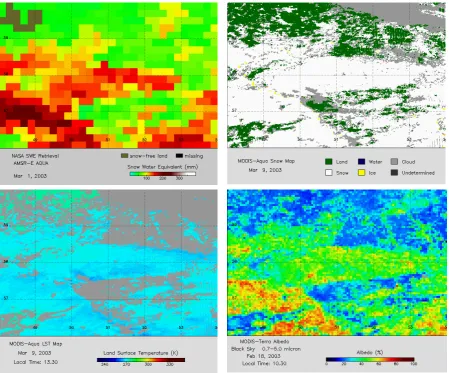
As an illustration of the obtained results, temporal changes of the criteria NME and NRMSE are shown in Fig. 5 for 3 of 19 polygons.

One can see from Fig. 5 that NME and NRMSE are close to zero in the beginning of spring, then the both criteria in-crease in the period of intensive melt and return to small val-ues in the end of melt season. In general, the model allowed us to reproduce temporal changes of SCA for the open areas with satisfactory accuracy.

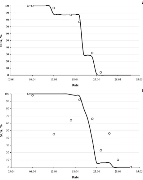
The accuracy of this reproduction is decreasing if we in-clude forested pixels in addition to open ones when SCA calculating. Figure 6 shows the temporal change of SCA for two polygons which are located correspondingly in the south-eastern and north-eastern corners of the study area and

Kilmez

-0.5 -0.3 -0.1 0.1 0.3 0.5

05.03 19.03 02.04 16.04 30.04

Date

NME

Kilmez

0 0.1 0.2 0.3 0.4 0.5

05.03 19.03 02.04 16.04 30.04

Date

NRMS

E

Kirov

-0.5 -0.3 -0.1 0.1 0.3 0.5

05.03 19.03 02.04 16.04 30.04

Date

NME

Kirov

0 0.1 0.2 0.3 0.4 0.5

05.03 19.03 02.04 16.04 30.04

Date

NRMS

E

Kirs

-0.5 -0.3 -0.1 0.1 0.3 0.5

05.03 19.03 02.04 16.04 30.04

Date

NME

Kirs

0 0.1 0.2 0.3 0.4 0.5

05.03 19.03 02.04 16.04 30.04

Date

NRMS

E

1 2 3 4 5 6 7

Fig. 5 Normalized mean error (NME) and normalized root mean square error (NRMSE) of simulated snow covered area in comparison with one obtained from NASA MOD10_L2 maps for three Thissen polygons surrounding meteorological stations Kilmez, Kirov, and Kirs (forested pixels are not taken into account ). 01/03/2002-30/04/2002

Fig. 5. Normalized mean error (NME) and normalized root

mean square error (NRMSE) of simulated snow covered area in comparison with one obtained from NASA MOD10 L2 maps for three Thissen polygons surrounding meteorological stations Kilmez, Kirov, and Kirs (forested pixels are not taken into account). 1 March 2002–30 April 2002.

have the coniferous forest percentage of 9% and 76% respec-tively. It can be seen from this Fig. 6 that, for the sparsely forested area the calculated values of SCA are close to the values defined from the satellite data while for the area with dense forest there is a significant difference between these values.

Daily maps of simulated snow characteristics were con-structed for the time period from 1 March to 30 June of 2002– 2005. Figure 7 presents the maps of simulated distributions of SWE for three dates in the second half of April 2003 cor-responding to the period of intensive snowmelt. These maps apparently present the spatial picture of snowmelt dynamics.

5 Using spatial snow characteristics for distributed

modelling of runoff generation in the Vyatka River basin

1 a 0 10 20 30 40 50 60 70 80 90 100

03.04 08.04 13.04 18.04 23.04 28.04 03.05

Date SC A, % b 0 10 20 30 40 50 60 70 80 90 100

03.04 08.04 13.04 18.04 23.04 28.04 03.05

Date SCA, % 2 3 4 5

Fig. 6. Changes of the calculated (line) and MODIS-based (points) SCA for two Thissen polygons with different cover percentages of coniferous forest (a - 9%; b – 76%).

a 0 10 20 30 40 50 60 70 80 90 100

03.04 08.04 13.04 18.04 23.04 28.04 03.05

Date SC A, % b 0 10 20 30 40 50 60 70 80 90 100

03.04 08.04 13.04 18.04 23.04 28.04 03.05

Date SCA, % 2 3 4 5

Fig. 6. Changes of the calculated (line) and MODIS-based (points) SCA for two Thissen polygons with different cover percentages of coniferous forest (a - 9%; b – 76%). Fig. 6. Changes of the calculated (line) and MODIS-based (points)

SCA for two Thissen polygons with different cover percentages of coniferous forest (a) 9%; (b) 76%).

model is based on the finite-element schematization of the basin and describes the processes of snow cover formation and snowmelt, freezing and thawing of soil, vertical moisture transfer and evaporation, surface water detention, overland, subsurface and channel flow. In the Vyatka River basin 477 area and 84 channel finite elements were defined taking into account the basin topography, soil properties, and vegetation type distribution as well as river channel structure and stream gage allocation (Fig. 8).

To calculate the characteristics of snow cover, Eqs. (1)– (26) were applied vertical water and heat transfer in the soil associated with soil freezing, thawing and infiltration of wa-ter is described with the following equations (Gelfan, 2006):

∂W ∂t = ∂ ∂z D∂θ

∂z+DI

∂I

∂z−K

(27) cT ∂T ∂t= ∂ ∂z λ∂T ∂z

+ρwcw

D∂θ

∂z+DI ∂I ∂z−K

_∂T

∂z+ρwL ∂W

∂t (28)

where W, θ and I represent the total water content, liq-uid water content and ice content of soil, respectively (W= θ+ρi

ρwI );K=K(θ,I )denotes the hydraulic conductivity of the frozen soil;T specifies the soil temperature;λrepresents

48 48.5 49 49.5 50 50.5 51 51.5 52 52.5 53 53.5 54 56 56.5 57 57.5 58 58.5 59 59.5 60 0 25 50 75 100 125 150 175 200 225 250 275 300 325 350 375 400 1 2

48 48.5 49 49.5 50 50.5 51 51.5 52 52.5 53 53.5 54 56 56.5 57 57.5 58 58.5 59 59.5 60 0 25 50 75 100 125 150 175 200 225 250 275 300 325 350 375 400 3 4

48 48.5 49 49.5 50 50.5 51 51.5 52 52.5 53 53.5 54 56 56.5 57 57.5 58 58.5 59 59.5 60 0 25 50 75 100 125 150 175 200 225 250 275 300 325 350 375 400 5 6 7 8

Fig. 7. The calculated maps of SWE (mm) (From the top to the bottom: 14, 19, 22 April, 2003).

Fig. 7. The calculated maps of SWE (mm) (From the top to the bottom: 14, 19, 22 April 2003).

the thermal conductivity of soil; D=K∂ψ_∂θ

I and DI

=

K∂ψ_∂I

θ;ψ

=ψ (θ,I )denotes the capillary potential of the

frozen soil;cT=ceff+ρwL_∂T∂θ;ceff represents the effective

heat capacity of soilceff=ρgcg(1−P )+ρwcwθ+ρiciI;ρ

andcspecify the density and the specific heat capacity, re-spectively (indexes w, i andg refer to water, ice and soil matrix, respectively);P represents the soil porosity.

1

2

3

4

Fig. 8. Finite-element schematization of the Vyatka River basin (bold lines represent the channel

network; thin lines represent the boundaries of finite elements; green labels mark the forested

elements).

Fig. 8. Finite-element schematization of the Vyatka River basin (bold lines represent the channel network; thin lines represent the boundaries of finite elements; green labels mark the forested ele-ments).

At the lower boundary of the podzol soils typical for the Vyatka River basin, there is an impermeable layer at the depth of 1–2 m. The vertical water flux is assumed zero at this boundary. It is also assumed that the horizontal move-ment of water along the impermeable layer occurs if the soil moisture content exceeds the field capacity,θf, of soil. As a

result, the horizontal flux,Rg, is calculated as:

Rg=

∂ ∂t

θ−θfzP (29)

wherezP is the soil layer in whichθ > θf.

The detention of melt water by depressions at the catch-ment surface is calculated by the formula assuming expo-nential distribution of the storage capacity (Kuchment et al., 1986).

The rate of evaporation from an unfrozen, snow-free soil is calculated by the formula presented by Kuchment et al. (2000).

The kinematic wave equations are applied to describe overland and subsurface flow. To account for the subsur-face flow, the following equations are used (Kuchment et al., 2000):

(P−θf)

∂h

∂t +

∂q

∂x=Rg (30)

q=Kgi0h

wherehis the subsurface flow depth;qis the subsurface flow discharge;i0is the slope of the layer with subsurface flow;

Kgis the horizontal hydraulic conductivity.

The kinematic wave equations are numerically integrated by the finite-element method coupled with the Galerkin method.

To calculate the water movement through the river channel elements, the advection-diffusion equation is applied. This equation was numerically integrated by the four-point im-plicit difference scheme.

To take into account subgrid effects, it was supposed that the saturated hydraulic conductivity is gamma-distributed within each finite element area. Mean value of this param-eter within a finite element was assessed using the available experimental measurement data for the different types of soil in the Vyatka River basin. Coefficient of variation within a finite element was determined from the empirical formula (Kuchment et al., 1986) which relates this coefficient to the mean value of the saturated hydraulic conductivity.

Most of the model parameters were assigned on the ba-sis of the available measurements of the basin characteristics including the basin topography and river channel data, soil, vegetation and snow constants as well as from empirical re-lationships that were derived and tested in (Kuchment et al., 2008) using mainly Russian experimental data and field ob-servations. Six parameters influencing the processes of in-filtration, soil moisture evaporation, detention in basin stor-age and flood routing were calibrated against the observed snowmelt flood hydrographs for the period from 1940 till 1959. Two parameters influencing snowmelt rate were cal-ibrated against snow measurements. The validation was car-ried out by comparison of the observed and simulated hy-drographs for the period from 1960 till 1980. The simulated and the observed hydrographs at the Vyatskie Polyany gage (the outlet gage of the Vyatka River basin) for the last ten years of the validation period are presented in Fig. 9. The standard deviation of errors of the simulated flood volumes and peak discharges are equal to correspondingly 1.1 km3 and 486 m3s−1. The Nash and Sutcliffe efficiency criterion for the flood volume and discharge simulations are 0.94 and 0.84, respectively.

1971 0 1000 2000 3000 4000 5000

17.02 19.03 18.04 18.05 17.06 17.07

Q, m3_{/s 1972}

0 1000 2000 3000 4000 5000 6000

17.02 19.03 18.04 18.05 17.06 17.07

1973 0 1000 2000 3000 4000 5000

17.02 19.03 18.04 18.05 17.06 17.07

1974 0 1500 3000 4500 6000 7500 9000

17.02 19.03 18.04 18.05 17.06 17.07

1975 0 1000 2000 3000 4000 5000 6000

17.02 19.03 18.04 18.05 17.06 17.07

1976 0 1000 2000 3000 4000 5000

17.02 19.03 18.04 18.05 17.06 17.07

1977 0 1000 2000 3000 4000 5000

17.02 19.03 18.04 18.05 17.06 17.07

1978 0 1000 2000 3000 4000

17.02 19.03 18.04 18.05 17.06 17.07

1979 0 1500 3000 4500 6000 7500 9000

17.02 19.03 18.04 18.05 17.06 17.07

1980 0 1000 2000 3000 4000 5000 6000

17.02 19.03 18.04 18.05 17.06 17.07

1 2

3

Fig. 9. Comparison of the observed (solid line) and calculated (dashed line) hydrographs at the gauge

Vyatskie Polyany of the Vyatka River (the last ten years of validation period). Fig. 9. Comparison of the observed (solid line) and calculated (dashed line) hydrographs at the gauge Vyatskie Polyany of the Vy-atka River (the last ten years of validation period).

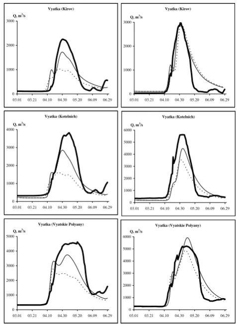
As a numerical experiment, we calculated snowmelt fields directly from the AE-DySno SWE maps and used these fields as inputs into the runoff generation model. It appears that the resulting hydrographs shown in Fig. 10 are significantly underestimated in comparison with the observed ones. This underestimation can be explained by large errors in satellite-derived SWE in forested areas and for snowpack saturated with melt water.

The obtained results can be viewed as an indication that characterization of snow cover fields by the proposed tech-nique can improve the representation of spatial distributions of SWE as compared to the respective fields obtained directly from satellite data. There is also an opportunity to fur-ther improve the accuracy of the proposed method using a more comprehensive calibration of the snowpack model with satellite measurements of SCA (if these data series are long enough) and the observed runoff hydrographs.

Vyatka (Vyatskie Polyany)

0 1000 2000 3000 4000 5000 6000

03.01 03.21 04.10 04.30 05.20 06.09 06.29

Q, m3/s

Vyatka (Kirov)

0 1000 2000 3000

03.01 03.21 04.10 04.30 05.20 06.09 06.29

Q, m3_/s

Vyatka (Kotelnich) 0 1000 2000 3000 4000 5000 6000

03.01 03.21 04.10 04.30 05.20 06.09 06.29

Q, m3/s

Vyatka (Vyatskie Polyany)

0 1000 2000 3000 4000 5000

03.01 03.21 04.10 04.30 05.20 06.09 06.29

Q, m3_/s

Vyatka (Kirov)

0 1000 2000 3000

03.01 03.21 04.10 04.30 05.20 06.09 06.29

Q, m3_/s

Vyatka (Kotelnich) 0 1000 2000 3000 4000

03.01 03.21 04.10 04.30 05.20 06.09 06.29

Q, m3_/s

1 2 3 4 5

Fig. 10. Comparison of the observed hydrographs (bold line) with the hydrographs calculated from the constructed SWE fields (thin line) and from AE-DySno SWE maps (dashed line). (The left column presents hydrographs of the 2003 flood, the right column presents hydrographs of the 2005 flood)

Fig. 10. Comparison of the observed hydrographs (bold line) with the hydrographs calculated from the constructed SWE fields (thin

line) and from AE-DySno SWE maps (dashed line). (The left

column presents hydrographs of the 2003 flood, the right column presents hydrographs of the 2005 flood).

6 Conclusions

The proposed technique may be useful for runoff simulation in river basins where the ground-based meteorological net-work is sparse and does not represent properly spatial hetero-geneities of snow characteristics. Because of large possible errors in satellite measurements of SWE during a snowmelt period, the satellite-derived SWE are used as the initial con-ditions. The correspondence of simulated and observed hy-drographs may be considered as an indicator of the accuracy of the constructed fields of snow characteristics and at the same time, as a measure of effectiveness of utilizing satellite-derived SWE data for runoff simulation. It is possible to as-sume that the suggested approach is especially designed to help physically based distributed hydrologic models realize their full potential in predicting spatial peculiarities of river runoff genesis.

Acknowledgements. This research is supported by NASA Grant

NNG06GH45G.

Edited by: J. Vrugt

References

Andreadis, K. M. and Lettenmaier, D. P.: Assimilating remotely sensed snow observations into a macroscale hydrology model, Adv. Water Resour., 6, 872–886, 2006.

Carroll, T., Cline, D., Olheiser, C., Rost, A., Nilsson, A., Fall, G., Bovitz, C., and Li, L.: NOAA national snow analysis. Proceed-ings of the 74th Annual Western Snow Conference, National Op-erational Hydrologic Remote Sensing Center, National Weather Service, NOAA, Chanhassen, Minnesota, 2–14, 2006.

Chang, A. T. C. and Rango, A.: Algorithm Theoretical Basis Doc-ument for the AMSR-E Snow Water Equivalent Algorithm, Ver-sion 3.1, Greenbelt, MD, USA, NASA Goddard Space Flight Center, 49 pp., 2000.

Dong, J., Walker, J. P., and Houser, P. R.: Factors affecting remotely sensed snow water equivalent uncertainty, Remote Sens. Envi-ron., 97, 68–82, 2005.

Dressler, K. A., Leavesley, G. H., Bales, R. C., and Fassnacht, S. R.: Evaluation of gridded snow water equivalent and satellite snow products for mountain basins in a hydrologic model, Hydrol. Pro-cess., 20, 673–688. 2006.

Engen, G., Guneriussen, T., Overrein, Ø.: Delta-K interferometric SAR technique for snow water equivalent (SWE) retrieval, IEEE Geosci. Remote S., 1(2), 57–61, 2004.

Foster, J., Hall, D., Eylander, J., Kim, E., Riggs, G., Tedesco, M., Nghiem, S., Kelly, R., Choudhury, B., and Reichle, R.: Blended visible, passive microwave and scatterometer global snow prod-ucts. Proc. 64th Eastern Snow Conf., St. Johns, Newfoundland, Canada 2007, 27–36, 2007.

Gelfan, A. N., Pomeroy, J. W., and Kuchment, L. S.: Modelling For-est Cover Influences on Snow Accumulation, Sublimation, and Melt, J. Hydrometeorol., 5, 785–803, 2004.

Gelfan, A. N.: Physically based model of heat and water transfer in frozen soil and its parametrization by basic soil data, in: Pre-dictions in Ungauged Basins: Promises and Progress, edited by: Sivapalan, M., Wagener, T., Uhlenbrook, S., Zehe, E., Lakshmi, V., Liang, X., Tachikawa, Y., and Kumar, P., IAHS Publication, Foz do Iguazu, Brazil, 303, 293–304, 2006.

Hall, D. K., Riggs, G., Salomonson, V., DiGirolamo, N. E., and Bayr, K. J.: MODIS snow cover products, Remote Sens. Envi-ron., 83, 181–194, 2002.

Hall, D. K. and Riggs, G.: Accuracy assessment of the MODIS snow products, Hydrol. Process., 21, 1534–1547, 2007

Hansen, M., DeFries, R., Townshend, J. R. G., and Sohlberg, R.: Global land cover classification at 1-km resolution using a deci-sion tree classifier, Int. J. Remote Sens., 21, 1331–1365, 2000. Kolberg, S., Rue, H., and Gottschalk, L.: A Bayesian spatial

assim-ilation scheme for snow coverage observations in a gridded snow model, Hydrol. Earth Syst. Sci., 10, 369–381, 2006,

http://www.hydrol-earth-syst-sci.net/10/369/2006/.

K¨onig, M., Winther, J. G., and Isacsson, E.: Measuring snow and glacier ice properties from satellite, Rev. Geophys., 39, 1–27, 2001.

Kuchment, L. S., Demidov, V. N., and Motovilov, Yu. G.: A phys-ically based model of the formation of snowmelt and rainfall runoff, IAHS Publication, 155, 27–36, 1986.

Kuchment, L. S. and Gelfan, A. N.: Physically based model of snow accumulation and melt in a forest, Meteorology and Hydrology, 5, 85–95, 2004 (in Russian).

Kuchment, L. S., Gelfan, A. N., and Demidov, V. N.: Assessments of magnitude and risk of dangerous floods on the basis of phys-ically based models of runoff generation. In: “Dangerous phe-nomena at the land surface: physical mechanisms and catas-trophic consequences” Published in the Institute of Geography of RAS, Moscow, Russia, 124–147, 2008 (in Russian).

Kuchment, L. S., Gelfan, A. N., and Demidov, V. N.: A distributed model of runoff generation in the permafrost regions, J. Hydrol., 240, 1–22, 2000.

Nosenko, O. A., Dolgih, N. A., and Nosenko, G. A.: Snow cover in the Central European Russia under the data derived from AMSR-E and SSM/I, in: “Recent problems of the land surface remote sensing from the space: physical basis, technologies of moni-toring of the environment and dangerous phenomena”, “Azbuka-2000”, Moscow, Russia, 296–301, 2006 (in Russian.)

Rodell, M. and Houser, P. R.: Updating a land surface model with MODIS-derived snow cover, J. Hydrometeorol., 5, 1064–1075, 2004.