https://doi.org/10.5194/hess-21-2649-2017 © Author(s) 2017. This work is distributed under the Creative Commons Attribution 3.0 License.
Scaled distribution mapping: a bias correction method that
preserves raw climate model projected changes
Matthew B. Switanek1, Peter A. Troch2, Christopher L. Castro2, Armin Leuprecht1, Hsin-I Chang2, Rajarshi Mukherjee2, and Eleonora M. C. Demaria3
1Wegener Center for Climate and Global Change, University of Graz, Graz, 8010, Austria
2Department of Hydrology and Atmospheric Sciences, University of Arizona, Tucson, Arizona 85721, USA 3Southwest Watershed Research Center, USDA – Agricultural Research Service, Tucson, Arizona 85719, USA Correspondence to:Matthew B. Switanek ([email protected])
Received: 25 August 2016 – Discussion started: 12 September 2016
Revised: 24 March 2017 – Accepted: 25 April 2017 – Published: 6 June 2017
Abstract.Commonly used bias correction methods such as quantile mapping (QM) assume the function of error cor-rection values between modeled and observed distributions are stationary or time invariant. This article finds that this function of the error correction values cannot be assumed to be stationary. As a result, QM lacks justification to in-flate/deflate various moments of the climate change signal. Previous adaptations of QM, most notably quantile delta mapping (QDM), have been developed that do not rely on this assumption of stationarity. Here, we outline a method-ology called scaled distribution mapping (SDM), which is conceptually similar to QDM, but more explicitly accounts for the frequency of rain days and the likelihood of individ-ual events. The SDM method is found to outperform QM, QDM, and detrended QM in its ability to better preserve raw climate model projected changes to meteorological variables such as temperature and precipitation.
1 Introduction
Bias correction of climate model projections is often per-formed in order to properly assess the impacts of climate change on human and environmental resources (Berg et al., 2003; Ines and Hansen, 2006; Muerth et al., 2013; Teng et al., 2015). Removing model bias is particularly useful for im-pact studies involving hydrological models, where runoff is a nonlinear function of precipitation (Christensen et al., 2008; Mauer and Hidalgo, 2008; Hagemann et al., 2011). Global climate models (GCMs) provide large-scale projections for
many climate variables (IPCC, 2013). However, many cli-mate processes and landscape features are not resolved at the coarse resolution of current GCMs. To bridge this gap, re-gional climate models (RCMs) are commonly used to down-scale GCM data to a higher resolution. Even though RCMs can provide added value (Fowler et al., 2007; Feser et al., 2011; Di Luca et al., 2013; Kotlarski, 2014), systematic er-rors in the model output still exist (Mearns et al., 2012; Sill-mann et al., 2013).
In this study, we focus specifically on the performance of bias correction and not issues related to downscal-ing/upscaling (Maraun, 2013). We have divided the study in two main sections: Sects. 3 and 4. In Sect. 3, first we begin by testing the stationarity assumption used in QM and the implications of this assumption. Second, we use a synthetic example to investigate the potential advantages of using a parametric instead of a non-parametric approach. Third, we illustrate the problems associated with validating bias correc-tion methods using a split-sample or cross-validacorrec-tion test. In Sect. 4, a new bias correction method called scaled distribu-tion mapping (SDM) is outlined. Finally, Sect. 5 compares and discusses the performances of SDM with other methods.
2 Data
Climate model data in this study use projections of daily mean temperature and precipitation values from the RACMO22E regional climate model. The KNMI-RACMO22E RCM was forced with the ICHEC-EC-EARTH GCM, and it is one of the model projec-tion runs in the EURO-CORDEX project. The data can be found on any of the ESGF repositories containing EURO-CORDEX (e.g., https://esgf-node.llnl.gov/projects/ esgf-llnl/). The model data for the years 1951–2005 and 2006–2100 correspond to the historical and RCP 8.5 (ESGF naming: r1i1p1) scenarios, respectively. Observational data for mean temperature and precipitation were obtained from the E-OBS data set (Haylock et al., 2008). The KNMI-RACMO22E climate data were upscaled from its original 0.11◦resolution to the 0.5◦E-OBS resolution.
3 Bias correction: methods, limitations, and evaluation
Over the years, numerous bias correction methods have been developed using univariate and multivariate approaches (Gellens and Roulin, 1998; Wood et al., 2004; Schmidli et al., 2006; Boé et al., 2007; Leander and Buishand, 2007; Lenderink et al., 2007; Li et al., 2010; Maraun et al., 2010; Piani et al., 2010; Themeßl et al., 2011; Piani and Haerter, 2012). In this study, we focus our study on univariate bias correction methods.
Many popular existing bias correction methods have been reviewed and compared and QM was found to outperform other methods (Gudmundsson et al., 2012; Teutschbein and Seibert, 2012, 2013; Chen et al., 2013). At the same time, studies have pointed out serious problems that arise when using QM for bias correction (Hagemann et al., 2011; The-meßl et al., 2012). In particular, the method can alter the raw model projected changes (Themeßl et al., 2012; Maurer and Pierce, 2014). This inflation or deflation of the raw simulated climate change signal exists as an artifact of the stationar-ity assumption. The impact that the stationarstationar-ity assumption
has on QM bias corrected data is discussed in more detail in Sect. 3.1.
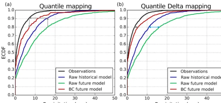
More recently, the standard non-parametric QM method has been adapted to more explicitly preserve the raw modeled climate change signals (Michelangeli et al., 2009; Olsson et al., 2009; Willems and Vrac, 2011; Sunyer et al., 2015; Wang and Chen, 2014; Cannon et al., 2015). Hempel et al. (2013) and Bürger et al. (2013) both used a form of detrended QM (DETQM) that better preserved monthly trends, but the daily values still are subject to the stationarity assumption, which can ultimately result in altering the raw modeled projected change. Extending previous work (e.g., Olsson et al., 2009; Bürger et al., 2013), Cannon et al. (2015) modified the QM method and outlined an approach called quantile delta map-ping (QDM). QDM is a break from other typical QM meth-ods insofar as that it is not constrained by the stationarity assumption. An example of QM versus QDM is shown in Fig. 1. In the traditional QM method, a raw modeled value is always corrected by the same value of bias or error that is determined by its respective quantile in the calibration pe-riod. On the other hand, QDM multiplies observed values by the ratio of the modeled values (period of interest di-vided by calibration period) at the same quantiles. Our pro-posed bias correction methodology, SDM, share some sim-ilarities with QDM; however, there are three important dis-tinctions: (1) SDM uses a parametric model instead of a non-parametric one, (2) SDM and QDM handle days with zero rainfall very differently, and (3) SDM more accurately ac-counts for the differences in the modeled variances, for tem-perature, between the period of interest and the calibration period.
3.1 Stationarity and quantile mapping
corre-Figure 1.Schematic of the quantile mapping versus quantile delta mapping methodologies. The red lines are the bias corrected values for the future model. The arrows in each panel illustrate the bias correction of a future modeled value at ECDF=0.8.
sponds to the quantile where ECDF equals 0.2, while at these same quantiles (ECDFs of 0.8 and 0.2), observations are 12 and 3◦C, respectively. Furthermore, the model is projecting more future values at 10◦C. As a result, QM will deflate or under-represent the raw model projected change. This is due to the fact that QM is more often using a 2◦C error correction value (12–10◦C, at ECDF of 0.8) instead of the 3◦C (3–0◦C, at ECDF of 0.2) correction.
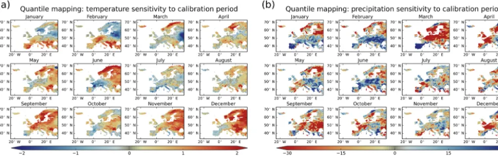
Altering of the raw model’s climate change signal could be justified with QM if one finds that the stationarity assumption is justified. We tested the stationarity assumption by investi-gating whether the error correction values are independent of the calibration period. To do this, the same daily data in the future time period (2071–2100) were bias corrected via stan-dard QM, separately for each month, using two different cali-bration periods (1951–1980 and 1976–2005). Figure 2 shows how sensitive QM is to using two different calibration peri-ods to bias correct these same future values. Figure 2a and b show the sensitivity for temperature and precipitation, re-spectively. There are instances where this sensitivity to the calibration period is nearly as large as the raw model pro-jected mean changes. This illustrates how unstable the error correction values in QM can be. If stationarity was a valid as-sumption, all the map colors in Fig. 2 would be much closer to gray. The calibration period largely influences the error correction values and, as a result, the stationarity assumption is invalid. As an additional test, we performed the bias cor-rection using a parametric implementation of QM and found the error correction values to be equally sensitive to the cho-sen calibration period.
The results shown in Fig. 2 have broad implications for QM. First, it shows that one cannot confidently correct a spe-cific modeled value with a spespe-cific error correction value. As an example, a raw modeled value of 50 mm can be corrected by−15 mm using one calibration period and+5 mm in an-other, leading to two very different bias corrected values of
35 and 55 mm, respectively. The effect that the calibration period has on QM can be mitigated to some extent by cali-brating on longer historical records (Teng et al., 2015). How-ever, one can never be sure that these error correction values have converged to be completely independent of time. Sec-ond, due to the fact that the error correction values in QM are not stationary, the altering of the climate change signal that results from this assumption is unjustified. Therefore, until some bias correction method provides proper justification to manipulate and alter the raw model projected climate change signal, a better performing method should strive to preserve the original projected changes.
3.2 Parametric versus non-parametric methodological approaches
[image:3.612.121.475.65.230.2]Figure 2.The sensitivity of quantile mapping (QM) to the calibration period. The same daily data in the future time period (2071–2100) was bias corrected, separately for each month, using two different calibration periods (1951–1980 and 1976–2005). Panels(a)and(b)show the sensitivity for temperature and precipitation, respectively. Gray reflects no sensitivity of QM to calibration period, while increased saturation of warmer and cooler colors depict non-stationary error correction values used by QM.
Figure 3.Synthetic data of observations (Obs) and modeled (Mod) data. Each data set consist of 200 values randomly sampled from the same gamma distribution with shape parameter equal to 0.8 and scale parameter equal to 12.0. Panel(a)shows the empirical distance (blue arrow) between the largest quantile of each distribution. Panel(b)shows the difference after fitting distributions and evaluating the largest events at the same cumulative distribution function (CDF) value (in this case the fitted CDF value of the observations).
(with the value of 32.8) corresponds to a fitted cumulative distribution function (CDF) of 0.993, while the largest quan-tile of Mod (with the value of 57.3) corresponds to a fitted CDF of 0.998. Using the fitted distributions, one can find the corresponding Mod value at the same expected Obs CDF of 0.993. In this example, that value is 44.8. Then our expected difference between events of the same expected probability has been reduced from 24.5 to 12.0 (where 24.5=57.3–32.8 and 12.0=44.8–32.8), depicted again as the blue line with arrows in Fig. 2b. With this one example case, it is impossi-ble to know if we are truly gaining information by accounting for differences in event likelihood.
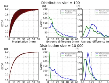
Figure 4 shows the results of a 1000 randomly gener-ated Obs and Mods values for distribution sizes of 100 and
dis-Figure 4.Observed (Obs) and modeled (Mods) values for distribution sizes of 100 and 10 000. As in Fig. 3, the values are randomly sampled from the same gamma distribution with shape parameter equal to 0.8 and scale parameter equal to 12.0. Panels(a)and(d)show the possible scenarios of ECDFs for the different distribution sizes. Panels(b)and(e)show the counts of the absolute differences between the extreme values using the non-parametric method (blue line) and the parametric method (green line). Similarly, panels(c)and(f)show the counts of the absolute differences, averaged over the entire distribution, between the values using the non-parametric and the parametric method.
tribution. However, with larger sample sizes, we are converg-ing on identical distributions for Obs and Mod. Therefore, the magnitude of the differences between extreme quantiles is simply due to sampling noise. On the other hand, if a dis-tribution is fit to the data first, then one gains information regarding the expected probabilities of specific events taking place with respect to the underlying distribution. This allows for the parametric method to reduce the error associated with sampling noise over that of the non-parametric method. 3.3 Validating bias correction methods
Split-sample or cross-validation tests are commonly used to validate how well bias correction methods perform un-der changing conditions (Maurer and Pierce, 2014; Klemeš, 1986; Wang and Chen, 2014; Piani et al., 2010). Typically, a period is chosen for calibrating the bias correction pa-rameters and then different bias correction methods’ perfor-mances are compared in a validation period. For example, bias correction parameters might be fit in a calibration pe-riod such as 1951–1980. Then, the performances of different methods are evaluated by comparing the bias corrected data to observations for the period 1981–2010. Unfortunately, split-sample tests that directly compare observations to bias corrected model data, for a time period outside of
calibra-tion, cannot distinguish between bias correction methodolog-ical performance and the performance of the underlying raw model. In this study. we define model performance by how well the raw model simulates changes to the statistical distri-bution of a climate variable with respect to observed changes to the distribution.
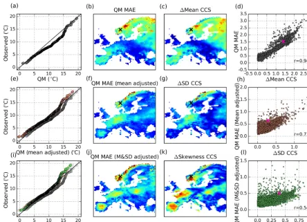
[image:5.612.119.475.64.337.2]Figure 5.Conflation of apparent bias correction skill (using QM) and model performance. The data are daily temperature values for the month of June for the period 1981–2010 after calibrating on the period 1951–1980. Panel(a)shows aQ−Qplot of an example grid cell delineated by the black X in the map panels and fuchsia scatter point in(d),(h), and(l). Panel(b)shows the mean absolute error (MAE) of theQ−Qplots from each grid cell, while(c)shows the raw model performance error of the mean. CCS refers to the climate change signal. Panel(d)shows the scatter and correlation between(b)and(c). The color maps of the second and third columns can be inferred from the scatter in the fourth column. After removing the raw model performance error of the mean, theQ−Qplot becomes the copper scatter in
(e). The QM MAE in(f)is the result of all the raw model mean performance errors being removed from each grid cell,(g)is the raw model performance error of the standard deviation, and(h)shows the scatter and correlation between(f), and(g). The raw model performance errors of the mean and the standard deviation are then removed, and theQ−Qplot becomes the green scatter in(i). After removing these errors for all grid cells, panels(j),(k)and(l)show the relationship between QM MAE and raw model performance error of the skewness.
shows the MAE values across all grid cells in the European domain. Figure 5c shows the model performance error of the mean, which is the difference between the raw model pro-jected mean temperature changes (1981–2010 with respect to 1951–1980) and the observed mean temperature changes (1981–2010 with respect to 1951–1980). It should be noted that the values in Fig. 5c are completely independent of any bias correction method being implemented; the values are solely dependent on observed and raw model values. Fig-ure 5d shows a scatter plot of the values corresponding to the grid cells in Fig. 5b and c. There is clearly a strong rela-tionship between the apparent performance of the QM, as it varies spatially, and how similar the raw modeled projected mean change is to the observed change. Most of the vari-ability pertaining to methodological performance (in a split-sample test) can be explained by the model performance
er-ror of the mean. If the raw modeled projected mean change in some grid cell is close to the observed change that took place (whether due to long-term forcing or internal climate variability), then it will appear that QM performs better in this grid cell, and vice versa.
(Fig. 5g). Again, much of the perceived method performance is simply due to how well the raw model simulated changes to the standard deviation (Fig. 5h). Fig. 5i–l further adjusts the QM bias corrected data by removing both the model per-formance errors from the mean and standard deviation. Still, there is a statistically significant relationship (p <0.01) be-tween method performance and the model performance error of the skewness.
Figure 5 illustrates how a split-sample or cross-validation test does not distinguish between methodological perfor-mance and raw model perforperfor-mance. Using pseudo-realities (Maraun et al., 2010) could tell us something more about the robustness of methods in different scenarios, but the per-formance of the bias correction method still cannot be sep-arated from how well individual models simulate raw pro-jected changes relative to the other models. In our example, we only looked at QM method performance and how this relates to model performance. Obviously, there will be dif-ferences from one bias correction method to another. How-ever, in a split-sample test, method and model performance are conflated. Consider a case, where a raw model projects changes across Europe that are 1◦C less than what was ob-served. Additionally, a particular bias correction method in-flates these projected changes by 1◦C, thereby canceling out the model performance error of the mean. It would appear that this particular method is performing better simply due to influence of model performance on validation.
Part of the validation procedure must ensure that the ob-served and modeled distributions in the calibration or his-torical period are statistically similar (Maraun et al., 2015). However, as shown here, validating bias corrected data in an-other period outside of the calibration period against obser-vations will not isolate bias correction methodological per-formance. Model performance will obscure the performance of the bias correction method. Instead, validation (or evalu-ation) should measure how well the raw modeled projected changes to the entire distribution are captured or preserved by the bias correction method between any two periods.
4 Scaled distribution mapping: method description and performance
Previous sections have shown that QM lacks justification for introducing inflation/deflation to the climate change signal (Sect. 3.1). This section introduces a bias correction method named SDM and its performance is compared to standard QM in addition to more recent and similar methods such as DETQM and QDM. Methodological performance is evalu-ated using raw model projected changes to the leading mo-ments (mean, standard deviation, and skewness) instead of individual quantiles because of our findings concerning the sampling noise associated with extreme values in the distri-butions (Sect. 3.2).
4.1 Scaled distribution mapping
A new bias correction methodology, called SDM, is pro-posed in this study. The conceptual framework of the method is quite similar to QDM (Fig. 1). However, as previously mentioned, our method has important differences that will be discussed in more detail in the “Performance” section (Sect. 4.2). The SDM method makes no assumption of sta-tionarity. It scales the observed distribution by raw model projected changes in magnitude, rain-day frequency (for pre-cipitation), and likelihood of events. The scaling changes as a function of the bias correction period. The next two sub-sections outline the SDM methodology for precipitation and temperature. Similar to other bias correction methods, a pre-screening of appropriate GCMs/RCMs is advised. Bias cor-rection will not, and should not, be expected to fix serious model deficiencies (garbage in – garbage out; e.g., Noguer et al., 1998). There are a few important differences between the implementation of SDM for precipitation and temperature. First, SDM scales the distribution of precipitation by a mul-tiplicative or relative amount and temperature is scaled by an absolute amount. Second, only values of positive precipita-tion exceeding a specified threshold (e.g., 0.1 mm) are used to build the distributions, while with temperature all values are used. Third, temperature data is first detrended, then bias corrected, and finally, the trends are added back in. As a re-sult, the variance is not inflated by temporal trends.
Bárdossy and Pegram (2012) showed that bias corrected data can still have systematic biases at different spatial scales. They illustrated that when raw modeled precipitation is less correlated across grid cells (lower average of its correlation matrix) than observations, the modeled extremes will be sys-tematically underestimated for larger spatial scales (averag-ing across tens to hundreds of grid cells) with respect to ob-servations. Similarly, an RCM with a higher average corre-lation matrix, with respect to observations, will overestimate extremes. We agree that this can be problematic for impact studies that rely on spatially distributed data across multiple grid cells (e.g., modeling hydrological extremes). In an ef-fort to properly reflect the statistical properties of the obser-vations in the calibration period at a variety of scales, we ad-vocate re-correlating the data (Bárdossy and Pegram, 2012) prior to implementing SDM.
4.1.1 Precipitation
fit a gamma distribution to the observed and modeled data for all grid cells. However, the gamma distribution will likely not be suitable for all studies involving precipitation, especially with respect to extremes (Papalexiou et al., 2013). Depend-ing on the type of analysis involved (e.g., changes to extreme precipitation, projected changes to the number of days with precipitation above 0.1 mm), the data should be fit with the distribution deemed most appropriate by the user. If a user does choose to fit a different distribution, that distribution can simply take the place of the gamma distribution outlined in the methodology. The SDM methodology for precipitation is now outlined in the following steps.
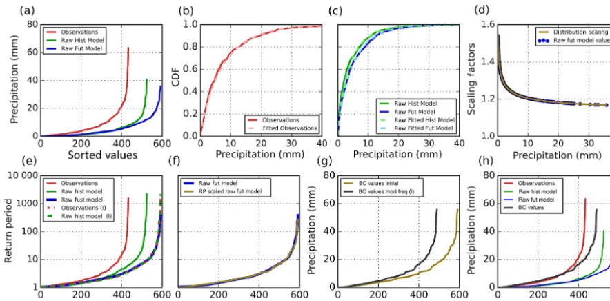
Step (1): set a raw modeled minimum precipitation thresh-old. In this study, we have used 0.1 mm as a threshold (which is the minimum amount of observed precipitation). When presenting the results, we additionally look at the impact of using a larger threshold of 1.0 mm. Any values below the threshold are set to 0.0 mm. Next, the days with precipitation are separated from days with no rainfall. Figure 6a shows the sorted values of precipitation for the observations, the raw historical model, and the raw future model. In this example, there are 434 observed rain days, 525 raw historical model rain days, and 593 raw future model rain days. Our expected number of bias corrected future model rain days, RDBC, can
be defined as RDBC=RDMODF×
RDOBSTDOBS
RDMODHTDMODH
, (1)
where TDOBS and TDMODH are the total number of days
including non-rain days for observations and raw historical model, while RDMODF, RDOBS, and RDMODHare the
num-ber of rain days for the raw model future, observations, and raw historical model. In this example, the total number of days including non-rain days is 900 for both the observa-tions and the raw historical model (30 years times 30 days in April). These lengths of days are included to allow for the flexibility of different calibration period lengths. Then, RDBC
is found to be 593×(434/900)/(525/900)=490 days (490 is the nearest integer value).
Step (2): fit gamma distribution parameters (or similarly the most appropriate distribution determined by the user), us-ing maximum likelihood, to the positive observed precipita-tion values (Fig. 6b), and the raw historical and future mod-eled values (Fig. 6c). The probability density function of the gamma distribution is
f (x;k, θ )=x
k−1exp −x θ
θk0 (k) , (2)
wherek(>0)is the shape parameter,θ (>0)is the scale pa-rameter,x(>0)is the precipitation amount, and0(k)is the gamma function evaluated atk. Next, use the fitted shape and scale parameters to find the corresponding CDF values of the positive precipitation events in the three time series. Set an upper threshold for the CDF values (e.g., 0.9999999), since
imprecise rounding can lead to the CDF function providing a value of 1.0, which corresponds to an infinite precipitation amount.
Step (3): calculate the scaling between the fitted raw future model distribution and the fitted raw historical distribution at all of the CDF values corresponding to the precipitation events of the raw future model time series. The scaling is calculated as
SFR=
ICDFMODF(CDFMODF)
ICDFMODH(CDFMODF)
, (3)
where SFRis an array of relative scaling factors (the length
is equal to number of rain days in the raw future model, which in this case is 593 values), ICDFMODFand ICDFMODH
are the inverse cumulative distribution functions (ICDFs), or the percent point functions, for the fitted future and histor-ical model distributions, respectively, while CDFMODF are
the estimated CDF values for the future raw model corre-sponding to the fitted distribution. The relative scaling fac-tors, for each raw future modeled value, can be seen in Fig. 6d. As an example, lets find the scaling factor that would correspond to the largest value in the raw future model time series. In the raw future model time series, this value is 35.8 mm. Using the fitted raw future model distribution, this event corresponds to a CDF value of 0.9974. The value ICDFMODF(0.9974)will yield the original value of 35.8 mm,
while ICDFMODH(0.9974)is equal to 30.6 mm. The most
ex-treme value that is bias corrected will have a relative scal-ing factor equal to 1.17 (35.8 mm/30.6 mm). For reference, the largest value in the raw historical model time series is 40.6 mm (seen in Fig. 6a). That value is more extreme with respect to its own distribution, with a corresponding CDF value of 0.9995. However, we want to compare events that are equally probable (as discussed in Sect. 3.3).
Step (4): calculate the recurrence intervals for the three sorted arrays of positive precipitation. The recurrence inter-val array, RI, is calculated as
RI= 1
1−CDF, (4)
Figure 6.Illustration of the scaled distribution mapping (SDM) methodology for precipitation. Panel(a)shows the sorted positive precipita-tion values for observaprecipita-tions, along with the raw historical and raw future model. Panels(b)and(c)show the empirical and fitted distributions. The scaling factors between the raw modeled future and historical time periods is shown in(d). The return periods and the scaled return pe-riod are plotted in(e)and(f), respectively (the (I) indicates the linear interpolation). Panel(g)shows the initial bias corrected precipitation values in gold and the final bias corrected values for the future model period is shown as the black line in(g)and(h).
Step (5): find the scaled or adjusted RI for the raw future model. This is calculated as
RISCALED=max
1,RIIOBS×RIMODF
RIIMODH
, (5)
where RIMODFis the RI for the raw future model and RIIOBS
and RIIMODH are the linearly interpolated RIs for the
ob-servations and raw historical model, respectively. The max-imum value, which is greater than or equal to 1, is used to evaluate each value in the RISCALED array. This is
neces-sary (especially for temperature) to ensure that the values of CDFSCALED in Eq. (6) are between 0 and 1. RISCALED
is shown in Fig. 6f as the gold line. This modifies or scales the RI of observed events by the projected changes to the ex-tremity of modeled events. RISCALED, for the most extreme
value, is found to be 321 days=1667×385/2000. As a re-sult, the return period of the most extreme observed value is reduced because the raw future modeled extreme value was more likely (smaller return period) than that of the raw his-torical modeled extreme value. Use the RISCALEDto find the
corresponding scaled CDF values with
CDFSCALED=1−
1 RISCALED
, (6)
where the CDFSCALED array is subsequently sorted in
de-scending order and reflects the scaling of the modeled change in event likelihood with respect to the observed likelihoods.
Step (6): the initial array of bias corrected values can now be calculated as
BCINITIAL=ICDFOBS(CDFSCALED)×SFR, (7)
where ICDFOBSis the inverse cumulative distribution
func-tion for the observed fitted distribufunc-tion, and CDFSCALEDand
SFR are obtained from Eqs. (6) and (3). Figure 6g shows
BCINITIALas the gold line. Lastly, the frequency of rain days
needs to be adjusted. Recall from Eq. (1), RDBCis equal to
490 days. BCINITIALis linearly interpolated from a length of
593 to 490 days. This yields the bias corrected values, which can be seen as the black line in Fig. 6h.
days than observations, that would have only translated to a 0.4 % reduction in total precipitation. This is due to the fact that the method is preferentially filling the largest events first. In the case that the historical model period and the bias correction period of interest completely overlap, the bias cor-rected data will be exactly the same as the observed distribu-tion. There would be no difference between the distributions in magnitude, likelihood, nor rain-day frequency, and there-fore the observed distribution undergoes no scaling.
4.1.2 Temperature
The SDM methodology for temperature is outline in the fol-lowing steps. Again, the future period is a general represen-tation of any time period one desires to bias correct, and it can be the same period as the raw historical model period.
Step (1): detrend the raw modeled and observed time se-ries in order to get a more accurate measure of the natural variability (we have used a linear trend, though any trend line could be used). These trends are added back in at the end, but until then, all subsequent steps use the detrended time series. Step (2): fit a normal probability distribution function to the detrended observed, raw historical modeled, and the raw future modeled time series. For a normal distribution, the fit-ted parameters are simply the empirical mean and standard deviation. Next, using these fitted normal distributions, find the corresponding CDF values for the temperature events that occurred in the three time series. Similarly to precipitation, set an upper and lower threshold for the CDF values (e.g., 0.0001, 0.9999). Again, imprecise rounding can lead to the CDF function providing a value of 1.0 or 0.0, which corre-sponds to an infinite temperature values.
Step (3): calculate the scaling between the fitted raw future model distribution and the fitted raw historical distribution at each probability of the events taking place in the raw future model time series. The scaling is then calculated as
SFA=[ICDFMODF(CDFMODF)−ICDFMODH(CDFMODF)]
×
σOBS σMODH
, (8)
where SFAis an array of absolute scaling factors, ICDFMODF
and ICDFMODHare again the ICDFs for the fitted future and
historical model distributions, CDFMODFis an array with the
estimated CDF values for the future raw model correspond-ing to the fitted distribution, andσOBS andσMODH are the standard deviations of the observed and raw historical distri-butions.
Step (4): next, calculate the recurrence intervals for the three sorted arrays of temperature with
RI= 1
0.5− |CDF−0.5|. (9)
Eq. (9) is different from Eq. (4) to reflect the two-tailed na-ture of a normal distribution.
Step (5): find RISCALED for the raw future model using
Eq. (5). If the lengths of the time series are the same for the historical and future periods, no linear interpolation is re-quired. Then, use the RISCALEDarray to find the
correspond-ing modified CDF values with
CDFSCALED=0.5+sgn(CDFOBS−0.5)
×
0.5− 1 RISCALED . (10)
Step (6): the initial array of bias corrected values can now be calculated as
BCINITIAL=ICDFOBS(CDFSCALED)+SFA, (11)
where all variables have been previously defined.
Step (7): reinsert the bias corrected values, BCINITIAL,
back into the correct temporal locations from the original raw future modeled time series. Lastly, the trend of the raw future modeled time series is added back into the bias cor-rected time series. Like with precipitation, when the histor-ical model period and the bias correction period of interest completely overlap, the bias corrected temperature data will be exactly the same as the observed distribution (except the trend of the bias corrected data will be that of the modeled trend and not of observations).
4.1.3 SDM and the temporal evolution of climate change
length of the sliding window to more/less strongly follow the raw modeled temporal evolution of climate change.
4.2 Performance
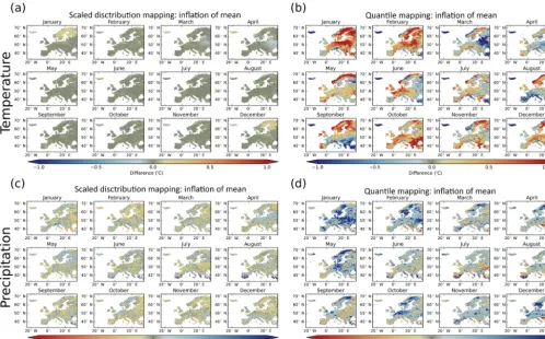
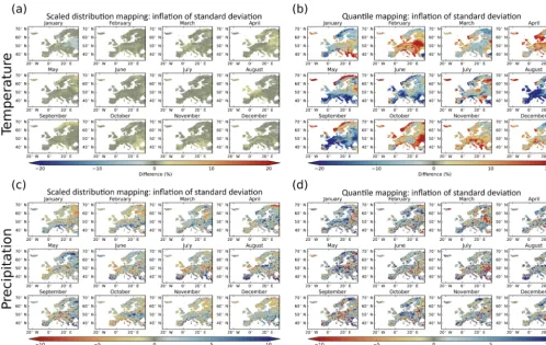
Figure 7 illustrates the amount of inflation (or deflation) that was introduced to the raw model projected change to the mean by the SDM and standard QM methods. The mean cli-mate change was evaluated between the periods 2071–2100 and 1971–2000. Figure 7a and b show the difference, by month, between the raw mean temperature changes and the bias corrected mean temperature changes when using SDM and QM, respectively. Similarly, Fig. 7c and d show the same but for relative change to precipitation. For both tempera-ture and precipitation, SDM has minimal inflation to the raw model projected mean change. In contrast, using QM leads to inflation greater than 1◦C and 10 %, for temperature and pre-cipitation, respectively, across large regions of Europe. Fig-ure 8 is the same as Fig. 7, but depicting the inflation of the standard deviation for SDM versus QM. Again, SDM much better preserves the raw model projected changes to the stan-dard deviation.
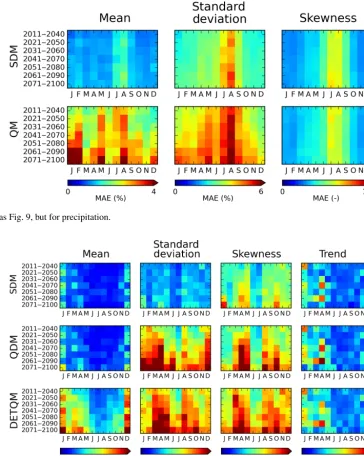
The temporal evolution of the SDM and QM performance, for all grid cells, is illustrated for temperature in Fig. 9. As discussed in Sect. 4.1.3, the authors implemented SDM us-ing 30-year periods with a 10-year slidus-ing window in order to bias correct the middle 10 years. The amount of infla-tion/deflation to the climate change signals is illustrated for the mean, standard deviation, skewness, and the trend. Each colored grid cell in the figure depicts the spatial MAE be-tween the raw model and bias corrected changes for all grid cells. For example, consider the lower left grid cell situated in the SDM row and mean column. This grid cell shows the spa-tial MAE between the raw modeled and bias corrected mean changes between the periods 2071–2100 and 1971–2000 for the month of January (it is the spatial MAE of the January panel of Fig. 7a). What is most noticeable is how the QM’s alteration (inflation/deflation) of the climate change signal increases as a function of the projected time period. When the projected period is furthest from the calibration period (2071–2100), the alteration to the leading three moments are the greatest. In contrast, SDM is seen to outperform QM in its ability to better preserve the raw projected changes. Fur-thermore, the performance of SDM does not degrade as a function of the projected time period. Figure 10 shows the same as Fig. 9, but for precipitation. Again, SDM performs much better in preserving the raw projected changes. This is especially true for projected changes to the mean and the standard deviation. It should be noted that all methods per-form worse for precipitation in the summer months. This can be explained by some regions (e.g., Spain) having very few days with precipitation, which cannot be fit well by either a parametric or a non-parametric method. Using a t test, the average MAEs for Figs. 9 and 10 (averaged over all months and outlook periods) are found to be statistically significantly
smaller for SDM versus the other three methods (p <0.01) for the leading three moments of the distribution.
Figure 11 compares the temperature performances of SDM to the more recent and similar methods of QDM and DETQM. SDM is seen to perform best with respect to bet-ter preserving the raw projected changes for the leading three moments of the distribution. Both SDM and QDM per-form equally well for preserving changes to the mean. How-ever, SDM better minimizes MAE for standard deviation and skewness. This can be attributed to one of the main differ-ences between the SDM and QDM methods. QDM scales the observed distribution by absolute difference between mod-eled quantiles (future – past), though this does not prop-erly scale the higher moments of the distribution. In con-trast, SDM applies the rightmost term, (σOBS/σMODH), in Eq. (8). This results in more appropriately scaling the higher moments of the bias corrected temperature data. The other difference between the methods is that SDM is parametric, while QDM is non-parametric or empirical.
Figure 12 compares the performances of the same three methods, but for precipitation. Again, SDM outperforms QDM and DETQM. Again, the average MAE for Figs. 11 and 12 are statistically significantly smaller for SDM (p <0.01) for the leading three moments of the distribution. In the case of precipitation, though, SDM shows the greatest improvement in its ability to preserve the raw projected mean change. This can be explained by the different ways that SDM, QDM, and DETQM handle days with zero precipitation. DETQM removes the mean modeled trend, but still performs poorly because the detrended error correction values are still assumed to be stationary. Like SDM, QDM implements a threshold of modeled precipitation. Then, these days of zero precipitation are filled with non-zero uniform random values below the trace threshold prior to bias correction. The multiplicative scaling amounts are subsequently found between all quantiles and applied to the observed quantiles. After bias correction, the values below the trace threshold are set back to zero. With that approach, the scaling is unstable when there is a mismatch in rain-day frequency. For example, consider a simplified example where the observed, raw future model and raw historical model have sorted arrays of precipita-tion amounts in millimeters of [0,1,4,15], [0,1,3,10], [0,0,1,8], respectively. After filling with uniform non-zero amounts, assume these arrays become [0.02,1,4,15], [0.04,1,3,10], [0.02,0.04,1,8]. The scaling array would then be [2,25,3,1.25]=[0.04,1,3,10]/[0.02,0.04,1,8]. Multiplying the scaling array by the observed ar-ray gives [0.04,25,12,18.75]. The raw mean change would then be 1.56=mean([0,1,3,10])
method-Figure 7.The amount of inflation (or deflation) introduced to the raw model projected change to the mean by the SDM and QM methods. The mean climate change was evaluated between the periods 2071–2100 and 1971–2000. Panels(a)and(b)show the monthly differences between the raw and bias corrected mean temperature changes using SDM and QM, respectively. Similarly,(c)and(d)show the same but for relative change to precipitation.
ology, linear interpolation is used to address the issue of different rain-day frequencies. This scales similar parts of the distribution and more explicitly changes the number of bias corrected rain days, and, as a result, SDM much better preserves raw modeled changes to the mean.
Additionally, we investigated the impact of using a differ-ent precipitation threshold. A precipitation value of 0.1 mm is very small and will have no noticeable impact for many applications. In those cases, it may be more appropriate to have a larger precipitation threshold. Figure 13 shows aver-age performances for each method when using a precipita-tion threshold of 0.1 and 1.0 mm, respectively. The perfor-mance of SDM improves as a result of using a larger thresh-old, while the performances of other methods remain ap-proximately the same. The improvement of SDM with the 1.0 mm threshold can be explained by the fact that a larger threshold leads to a better fit to the distribution. For obser-vations, averaged across all grid cells, we found that precip-itation amounts of less than 1.0 mm (and>=0.1 mm) made up 21.6 % of all positive precipitation days, while the sum of these low values only comprised 2.4 % of the total pre-cipitation. Similarly for the modeled data, 41.3 % of all
posi-tive precipitation days had precipitation amounts of less than 1.0 mm (and >=0.1 mm), which cumulatively comprised 5.4 % of the total precipitation. As a result, we found that using a smaller threshold can adversely affect the quality of the fit especially with respect to the extremes.
5 Conclusions
[image:12.612.51.550.66.376.2]Figure 8.Same as Fig. 7, but depicting the inflation of the standard deviation for SDM versus QM.
[image:13.612.90.507.456.640.2]Figure 10.Same as Fig. 9, but for precipitation.
Figure 11.Same as Fig. 9, but compares the temperature performances of SDM to the more recent and similar methods of QDM and DETQM.
as such? These are difficult questions, and more reflection and investigation is required before we find answers that are indisputable. In any regard, for the foreseeable future, there will continue to be scientists that use bias correction methods for impact assessment studies.
Statistical bias correction methods vary considerably and can have a large influence on the expected regional impacts of climate change. Multiple studies have previously come to the conclusion that QM is one of the better existing bias cor-rection methods (Gudmundsson et al., 2012; Teutschbein and Seibert, 2012, 2013; Chen et al., 2013). However, our anal-ysis highlighted two issues that challenge this conclusion.
First, we demonstrated that the stationarity assumption is in-valid and, as a result, the climate change signal cannot be justifiably altered using QM. Second, split-sample or cross-validation evaluation tests do not isolate the performance of the bias correction methods themselves. These performances are conflated with how well the raw model(s) simulate the observed changes to the leading moments of the distribution. In light of these issues, the performance of a bias correc-tion method should be validated on how well it preserves raw model projected changes across the entire distribution.
Figure 12.Same as Fig. 10, but compares the precipitation performances of SDM to the more recent and similar methods of QDM and DETQM.
[image:15.612.121.476.429.663.2]model projected changes to magnitude, rain-day frequency (for precipitation), and the likelihood of events. The perfor-mance of SDM was evaluated and found to perform better than traditional QM along with recent methods that are more similar such as QDM and DETQM. We advocate using a bias correction method, such as SDM, which scales the observed distribution by simulated changes across the modeled distri-bution. As a result, one need not rely on the invalid station-arity assumption.
Code and data availability. The data are available at ESGF (e.g., https://esgf-node.llnl.gov/projects/esgf-llnl/) and the python codes for running the SDM methodology are available upon request from the corresponding author. A reference implementation can be ob-tained from https://github.com/wegener-center/pyCAT.
Competing interests. The authors declare that they have no conflict of interest.
Acknowledgements. The work was supported by the project ÖKS15, funded by the Austrian Federal Ministry of Agriculture, Forestry, Environment and Water Management. The authors had additional support from the United States Bureau of Reclamation, and the federal state government of Austria with the projects CHC-FloodS (id: B368584) and DEUCALION II (id: B464795), both funded by the Austrian Klima- und Energiefonds through the Austrian Climate Research Program (ACRP). We acknowledge the World Climate Research Programme’s Working Group on Regional Climate, and the Working Group on Coupled modeling, former coordinating body of CORDEX and responsible panel for CMIP5. We also thank the climate modeling groups (Royal Netherlands Meteorological Institute (KNMI)) for producing and making available their model output. We also acknowledge the Earth System Grid Federation infrastructure an international effort led by the U.S. Department of Energy’s Program for Climate Model Diagnosis and Intercomparison, the European Network for Earth System modeling, and other partners in the Global Organisation for Earth System Science Portals (GO-ESSP). We acknowledge the E-OBS data set from the EU-FP6 project ENSEMBLES (http://ensembles-eu.metoffice.com) and the data providers in the ECA&D project (http://www.ecad.eu). The authors acknowledge the computing time granted by the John von Neumann Institute for Computing (NIC) and provided on the supercomputer JURECA at Jülich Supercomputing Centre (JSC). Finally, we gratefully acknowledge the helpful comments and suggestions of Douglas Maraun.
Edited by: E. Zehe
Reviewed by: U. Ehret and A. Bàrdossy
References
Bárdossy, A. and Pegram, G.: Multiscale spatial recorrelation of RCM precipitation to produce unbiased climate change scenar-ios over large areas and small, Water Resour. Res., 48, W09502, https://doi.org/10.1029/2011WR011524, 2012.
Berg, A. A., Famiglietti, J. S., Walker, J. P., and Houser, P. R.: Im-pact of bias correction to reanalysis products on simulations of north american soil moisture and hydrological fluxes, J. Geo-phys. Res., 108, 4490, https://doi.org/10.1029/2002JD003334, 2003.
Boé, J., Terray, L., Habets, F. and Martin, E.: Statistical and dynamical downscaling of the Seine basin climate for hydro-meteorological studies, Int. J. Climatol., 27, 1643–1655, https://doi.org/10.1002/joc.1602, 2007.
Brekke, L., Thrasher, B., Maurer, E. P., and Pruitt, T.: Downscaling CMIP3 and CMIP5 climate projections: Release of downscaled CMIP5 climate projections, comparison with preceding informa-tion, and summary of user needs, US Dept. of Interior, Bureau of Reclamation, Denver, CO, 104 pp., 2013.
Bürger, G., Sobie, R., Cannon, A. J., Werner, A. T., and Mur-dock, T. Q.: Downscaling extremes: An intercomparison of mul-tiple methods for future climate, J. Climate, 26, 3429–3449, https://doi.org/10.1175/JCLI-D-12-00249.1, 2013.
Cannon, A. J., Sobie, S. R., and Murdock, T. Q.: Bias correction of GCM precipitation by quantile mapping: How well do meth-ods preserve changes in quantiles and extremes?, J. Climate, 28, 6938–6959, https://doi.org/10.1175/JCLI-D-14-00754.1, 2015. Chen, J., Brissette, F. P., Chaumont, D., and Braun, M.:
Perfor-mance and uncertainty evaluation of emprirical downscaling methods in quantifying the climate impacts on hydrology over two North American river basins, J. Hydrol., 479, 200–214, https://doi.org/10.1016/j.jhydrol.2012.11.062, 2013.
Christensen J. H., Boberg, F., Christensen, O. B., and Lucas-Picher, P.: On the need for bias correction of regional climate change projections of temperature and precipitation, Geophys. Res. Lett., 35, L20709, https://doi.org/10.1029/2008GL035694, 2008.
Di Luca, A., de Elía, R. and Laprise, R.: Potential for small scale added value of RCM’s downscaled climate change signal, Clim. Dynam., 40, 601–618, doi:10.1007/s00382-012-1415-z, 2013. Ehret, U., Zehe, E., Wulfmeyer, V., Warrach-Sagi, K., and Liebert,
J.: HESS Opinions “Should we apply bias correction to global and regional climate model data?”, Hydrol. Earth Syst. Sci., 16, 3391–3404, https://doi.org/10.5194/hess-16-3391-2012, 2012. Feser, F., Rockel, B., von Storch, H., Winterfeldt, J., and Zahn, M.:
Regional climate models add value to global model data: a review and selected examples, B. Am. Meteorol. Soc., 92, 1181–1192, https://doi.org/10.1175/2011BAMS3061.1, 2011.
Fowler, H. J., Blenkinsop, S., and Tebaldi, C.: Linking climate change modelling to impacts studies: recent advances in down-scaling techniques for hydrological modelling, Int. J. Climatol., 27, 1547–1578, https://doi.org/10.1002/joc.1556, 2007. Gellens, D. and Roulin, E.: Streamflow response of Belgian
catch-ments to IPCC climate change scenarios, J. Hydrol., 210, 242– 258, https://doi.org/10.1016/S0022-1694(98)00192-9, 1998. Gudmundsson, L., Bremnes, J. B., Haugen, J. E., and
com-parison of methods, Hydrol. Earth Syst. Sci., 16, 3383–3390, https://doi.org/10.5194/hess-16-3383-2012, 2012.
Hagemann, S., Chen, C., Haerter, J. O., Heinke, J., Gerten, D., and Piani, C.: Impact of a statistical bias correction on the projected hydrological changes obtained from three GCMs and two hydrology models, J. Hydrometeorol., 12, 556–578, https://doi.org/10.1175/2011JHM1336.1, 2011.
Haylock, M. R., Hofstra, N., Klein Tank, A. M. G., Klok, E. J., Jones, P. D., and New, M.: A European daily high-resolution gridded dataset of surface temperature and precipitation, J. Geophys. Res.-Atmos., 113, D20119, https://doi.org/10.1029/2008JD10201, 2008.
Hempel, S., Frieler, K., Warszawski, L., Schewe, J., and Piontek, F.: A trend-preserving bias correction – the ISI-MIP approach, Earth Syst. Dynam., 4, 219–236, https://doi.org/10.5194/esd-4-219-2013, 2013.
Ines, A. V. M. and Hansen, J. W.: Bias correction of daily GCM rainfall for crop simulation studies, Agr. Forest Meteorol., 138, 44–53, https://doi.org/10.1016/j.agrformet.2006.03.009, 2006. IPCC: Climate Change 2013: The Physical Science Basis.
Con-tribution of Working Group I to the Fifth Assessment Re-port of the Intergovernmental Panel on Climate Change, edited by: Stocker, T. F., Qin, D., Plattner, G.-K., Tignor, M., Allen, S. K., Boschung, J., Nauels, A., Xia, Y., Bex, V., and Midgley, P. M., Cambridge University Press, Cam-bridge, United Kingdom and New York, NY, USA, 1535 pp., https://doi.org/10.1017/CBO9781107415324, 2013.
Klemeš, V.: Operational testing of hydrological simulation models/V(e)rification, en conditions r(e)elles, des mod(e)les de simulation hydrologique, Hydrol. Sci. J., 31, 13–24, https://doi.org/10.1080/02626668609491024, 1986.
Kotlarski, S., Keuler, K., Christensen, O. B., Colette, A., Déqué, M., Gobiet, A., Goergen, K., Jacob, D., Lüthi, D., van Meij-gaard, E., Nikulin, G., Schär, C., Teichmann, C., Vautard, R., Warrach-Sagi, K., and Wulfmeyer, V.: Regional climate model-ing on European scales: a joint standard evaluation of the EURO-CORDEX RCM ensemble, Geosci. Model Dev., 7, 1297–1333, https://doi.org/10.5194/gmd-7-1297-2014, 2014.
Leander, R., Buishand, T. A., van den Hurk, B. J. J. M., and de Wit, M. J. M.: Estimated changes in flood quantiles of the river Meuse from resampling of regional climate model output, J. Hydrol., 351, 331–343, https://doi.org/10.1016/j.jhydrol.2007.12.020, 2008.
Lenderink, G., Buishand, A., and van Deursen, W.: Estimates of fu-ture discharges of the river Rhine using two scenario methodolo-gies: direct versus delta approach, Hydrol. Earth Syst. Sci., 11, 1145–1159, https://doi.org/10.5194/hess-11-1145-2007, 2007. Li, H., Sheffield, J., and Wood, E. F.: Bias correction of
monthly precipitation and temperature fields from Intergovern-mental Panel on Climate Change AR4 models using equidis-tant quantile matching, J. Geophys. Res., 115, D10101, https://doi.org/10.1029/2009JD012882, 2010.
Maraun, D.: Nonstationarities of regional climate model biases in European seasonal mean temperature and precipitation sums, Geophys. Res. Lett., 39, L06706, https://doi.org/10.1029/2012GL051210, 2012.
Maraun, D.: Bias correction, quantile mapping, and downscal-ing: Revisiting the inflation issue, J. Climate, 26, 2137–2143, https://doi.org/10.1175/JCLI-D-12-00821.1, 2013.
Maraun, D., Wetterhall, F., Ireson, A. M., Chandler, R. E., Kendon, E. J., Widmann, M., Brienen, S., Rust, H. W., Sauter, T., The-meßl, M., Venema, V. K. C., Chun, K. P., Goodess, C. M., Jones, R. G., Onof, C., Vrac, M., and Thiele-Eich, I.: Precipita-tion downscaling under climate change: Recent developments to bridge the gap between dynamical models and the end user, Rev. Geophys., 48, RG3003, https://doi.org/10.1029/2009RG000314, 2010.
Maraun, D., Widmann, M., Gutierrez, J. M., Kotlarski, S., Chan-dler, R. E., Hertig, E., Wibig, J., Huth, R., and Wilcke, R. A. I.: VALUE: A framework to validate downscaling ap-proaches for climate change studies, Earth’s Future, 3, 1–14, https://doi.org/10.1002/2014EF000259, 2015.
Maurer, E. P. and Hidalgo, H. G.: Utility of daily vs. monthly large-scale climate data: an intercomparison of two statistical downscaling methods, Hydrol. Earth Syst. Sci., 12, 551–563, https://doi.org/10.5194/hess-12-551-2008, 2008.
Maurer, E. P. and Pierce, D. W.: Bias correction can modify cli-mate model simulated precipitation changes without adverse ef-fect on the ensemble mean, Hydrol. Earth Syst. Sci., 18, 915– 925, https://doi.org/10.5194/hess-18-915-2014, 2014.
Maurer, E. P., Das, T., and Cayan, D. R.: Errors in climate model daily precipitation and temperature output: time invariance and implications for bias correction, Hydrol. Earth Syst. Sci., 17, 2147–2159, https://doi.org/10.5194/hess-17-2147-2013, 2013. Mearns, L. O., Arritt, R., Biner, S., Bukovsky, M. S., McGinnis,
S., Sain, S., Caya, D., Correia Jr., J., Flory, D., Gutowski, W., Takle, E. S., Jones, R., Leung, R., Moufouma-Okia, W., Mc-Daniel, L, Nunes, A. M. B., Qian, Y., Roads, J., Sloan, L., and Snyder, M.: The North American regional climate change as-sessment program: Overview of phase I results, B. Am. Mete-orol. Soc., 93, 1337–1362, https://doi.org/10.1175/BAMS-D-11-00223.1, 2012.
Michelangeli, P. A., Vrac, M., and Loukos, H.: Probabilis-tic downscaling approaches: Application to wind cumula-tive distribution functions, Geophys. Res. Lett., 35, L11708, https://doi.org/10.1029/2009GL038401, 2009.
Muerth, M. J., Gauvin St-Denis, B., Ricard, S., Velázquez, J. A., Schmid, J., Minville, M., Caya, D., Chaumont, D., Lud-wig, R., and Turcotte, R.: On the need for bias correction in regional climate scenarios to assess climate change im-pacts on river runoff, Hydrol. Earth Syst. Sci., 17, 1189–1204, https://doi.org/10.5194/hess-17-1189-2013, 2013.
Noguer, M., Jones, R., and Murphy, J.: Sources of systematic er-rors in the climatology of a regional climate model over Europe, Clim. Dynam., 14, 691–712, 1998.
Olsson, J., Berggren, K., Olofsson, M. and Viklander, M.: Apply-ing climate model precipitation scenarios for urban hydrological assessment: A case in Kalmar City, Sweden, Atmos. Res., 92, 364–375, https://doi.org/10.1016/j.atmosres.2009.01.015, 2009. Papalexiou, S. M., Koutsoyiannis, D., and Makropoulos, C.:
How extreme is extreme? An assessment of daily rain-fall distribution tails, Hydrol. Earth Syst. Sci., 17, 851–862, https://doi.org/10.5194/hess-17-851-2013, 2013.
Piani, D. and Haerter J. O.: Two-dimensional bias correction of tem-perature and precipitation copulas in climate models, Geophys. Res. Lett., 39, L20401, https://doi.org/10.1029/2012GL053839, 2012.
Pierce, D. W., Cayan, D. R., Das, T., Maurer, E. P., Miller, N. L., Bao, Y., Kanamitsu, M., Yoshimura, K., Snyder, M. A., Sloan, L. C., Franco, G., and Tyree, M.: The key role of heavy precip-itation events in climate model disagreements of future annual precipitation changes in California, J. Climate, 26, 5879–5896, https://doi.org/10.1175/jcli-d-12-00766.1, 2013.
Schmidli, J., Frei, C., and Vidale, P. L.: Downscaling from GCM precipitation: a benchmark for dynamical and statis-tical downscaling methods, Int. J. Climatol., 26, 679–689, https://doi.org/10.1002/joc.1287, 2006.
Sillmann, J., Kharin, V., Zhang, X., Zwiers, F., and Bronaugh, D.: Climate extremes indices in the CMIP5 multimodel ensemble: Part 1. Model evaluation in the present climate, J. Geophys. Res.-Atmos., 118, 1716–1733, https://doi.org/10.1002/jgrd.50203, 2013.
Sunyer, M. A., Hundecha, Y., Lawrence, D., Madsen, H., Willems, P., Martinkova, M., Vormoor, K., Bürger, G., Hanel, M., Kri-auciuniene, J., Loukas, A., Osuch, M., and Yücel, I.: Inter-comparison of statistical downscaling methods for projection of extreme precipitation in Europe, Hydrol. Earth Syst. Sci., 19, 1827–1847, https://doi.org/10.5194/hess-19-1827-2015, 2015. Teng, J., Potter, N. J., Chiew, F. H. S., Zhang, L., Wang, B.,
Vaze, J., and Evans, J. P.: How does bias correction of regional climate model precipitation affect modelled runoff?, Hydrol. Earth Syst. Sci., 19, 711–728, https://doi.org/10.5194/hess-19-711-2015, 2015.
Teutschbein, C. and Seibert, J.: Bias correction of regional climate model simulations for hydrological climate-change impact stud-ies: Review and evaluation of different methods, J. Hydrol., 456– 457, 12–29, https://doi.org/10.1016/j.jhydrol.2012.05.052, 2012. Teutschbein, C. and Seibert, J.: Is bias correction of re-gional climate model (RCM) simulations possible for non-stationary conditions?, Hydrol. Earth Syst. Sci., 17, 5061–5077, https://doi.org/10.5194/hess-17-5061-2013, 2013.
Themeßl, M., Gobiet, A., and Leuprecht, A.: Empirical statis-tical downscaling and error correction of daily precipitation from regional climate models, Int. J. Climatol., 31, 2087–2105, https://doi.org/10.1007/s00382-010-0979-8, 2011.
Themeßl, M., Gobiet, A., and Heinrich, G.: Empirical-statistical downscaling and error correction of regional climate models and its impact on the climate change signal, Climate Change, 112, 449–468, https://doi.org/10.1007/s10584-011-0224-4, 2012. Wang, L. and Chen, W.: Equiratio cumulative distribution
func-tion matching as an improvement to the equidistant approach in bias correction of precipitation, Atmos. Sci. Lett., 15, 1–6, https://doi.org/10.1002/asl2.454, 2014.
Willems, P. and Vrac, M.: Statistical precipitation down-scaling for small-scale hydrological impact investiga-tions of climate change, J. Hydrol., 402, 193–205, https://doi.org/10.1016/j.jhydrol.2011.02.030, 2011.