A Two-Phase Hybrid Particle Swarm Optimization
Algorithm for Solving Permutation Flow-Shop
Scheduling Problem
Ko-Wei Huang
Institute of Computer and
Communication Engineering,
Department of Electrical
Engineering,National Cheng
Kung University, Tainan 70101,
Taiwan, ROC.
Chu-Sing Yang
Institute of Computer and
Communication Engineering,
Department of Electrical
Engineering,National Cheng
Kung University, Tainan 70101,
Taiwan, ROC.
Chun-Wei Tsai
Department of Applied
Geoinformatics,
Chia Nan University of
Pharmacy Science, Tainan
71710, Taiwan, ROC
ABSTRACT
In this paper, a two-phase hybrid particle swarm optimization algorithm (PRHPSO) is proposed for the permutation flow-shop scheduling problem (PFSP) with the minimizing makespan measure. The smallest position value (SPV) rule is used for encoding the particles that enable PSO for suitable PFSP, and the NEH and Tabu search algorithms are used for initializing the particles. In the first phase, the pattern reduction (PR) operator is used in the PSO algorithm for reducing the computation time. In order to avoid a premature convergence, a regeneration operator is used for escaping to the local optimal and balancing exploitation and exploration in the second phase. Additionally, a simulated annealing (SA) algorithm is utilized for local search to improve the best solution after the PSO search process. Finally, the results show that PRHPSO is significantly faster than two PSO-based algorithms and presents large-sized benchmarks.
General Terms
Hybrid Metaheuristic Algorithm, Combinatorial optimization.
Keywords
Particle swarm optimization, Permutation flow-shop scheduling problem, Pattern reduction, Makespan, Pattern Reduction, Regeneration Operator.
1.
INTRODUCTION
Johnson [1] pioneered permutation flow-shop problem research in 1953. Since then, the flow-shop scheduling problem (PFSP), an NP-hard problem, has received increasing attention in the combinatorial optimization research community. Rinnooy Kan [2] proved that minimizing the makespan was an NP-hard problem, and Garay et al. [3] proved that total flow-time minimization was also an NP-hard problem. Non-polynomial computing time is required for finding solutions. The objective of the PFSP is to find the sequence of jobs being processed in all machines to optimize the performance measure. Heuristics algorithms are commonly used for obtaining approximate solutions and decreasing CPU time in NP-hard combinatorial optimization problems. By 1983, the Nazwa-Enscore-Ham (NEH) [4] heuristics had been a well-known algorithm for makespan minimization for more than twenty-years.
Table 1: Examples permutation flowshop solution
Solution Redundant sub-solution
1234567
123 1235467
1236457 1234765 1236574
The PFSP is defined as follows. Considering n jobs{ 𝑗1, 𝑗2, 𝑗3, … , 𝑗𝑛}with each job successively processed by
mmachines{ 𝑀1, 𝑀2, 𝑀3, … , 𝑀𝑚}, the processing time is given
by𝑝𝑖,𝑘 between job i and machine k. On the other hand, there
are rule restrictions in the PFSP that each machine is permitted processing one job at most, and each job can be processed on one machine at any time. The goal of the PFSP is to find the best sequence (order or permutation) of jobs and optimize the object function. There are two common object functions in PFSP, namely makespan and total flow-time minimization.It is given that𝜋 = { 𝑗1, 𝑗2, 𝑗3, … , 𝑗𝑛}, which
indicates the job sequence, andC 𝑗𝑖, 𝑘 , denotes the
completion time of job i on machine k. C 𝑗𝑖, 𝑘 can be defined as Eq. 1.
The objective of the makespan is to find permutation 𝜋𝑏𝑒𝑠𝑡in
permutation set Π, such that Eq. 2 shows:
population-based heuristic approaches (such like PSO, GA, DE…etc.) all share the same critical problem when populations evolve over a period of time. For example, five solutions are obtained as shown in Table. 1. Each solution contains sub-solution 123 at the same position, meaning that it would spend redundant CPUcomputation time on calculating the makespan with sub-solution 123. If redundant calculations can be removed, the CPU computation time can be greatly reduced.This paper proposes a two-phaseparticle swarm optimization algorithm for solving permutation flow-shop scheduling problems. The most significant concerns are decreasing computation time and increasing the diversity of solutions. The algorithm has two tasks.
a) To eliminate redundant computations and reduce total computation time.
b) To enhance search behaviour and improve solution quality. The task is divided into two parts. Common sub-solutions are detected and compressed in part 1, while the regeneration operator is used for preserving exploitation and exploration when all solutions have the same job sequence in part 2. To improve the quality after the two-phase PSO algorithm, the SA-based local search is used for fine-tuning the solution, which is the simulated annealing (SA) [18] combined with the variable neighborhood local search [19]. The experimental results show that the algorithms are significantly faster than two recently proposed PSO-based algorithms using a different scale of benchmarks.
The remainder of this paper is organized as follows. Background knowledge and related work are described in Section 2. Section 3 states the details of the proposed algorithms. Evaluations of the proposed algorithms are described in Section 4. Finally, conclusions and future work are described in Section 5.
2.
BACKGROUND AND RELATED
WORK
In this section, the background of this research field and the related study are reviewed. The overview will focus on four main topics of
a) NEH heuristic algorithm (NEH), b) Tabu Search (TS),
c) Simulated Annealing (SA), and d) Particle Swarm Optimization (PSO).
2.1
NEH Heuristic algorithm
For more than, the Nawaz-Enscore-Ham (NEH) [4] heuristic algorithm has a widely-used algorithm for solving the makespan minimization problem. The NEH algorithm is divided into three parts.
1. Each job is sorted in descending order of processing time on the machines.
2. The first two jobs are chosen. A better partial order is obtained by scheduling them according to a comparison of makespan values.
3. Job j = 3,…, n, is inserted at each of j’s possible positions in the sequence to obtain the best partial schedule which minimizes the partial makespan.
Although the NEH heuristics is easy to implement, its time complexity is O 𝑛3𝑚 . Many studies have proposed ways to
improve the quality or computation time of the original NEH heuristic, such as [20][21][22].
2.2
Tabu Search
Tabu (also called Taboo) search (TS), which was proposed by Glover et al. [23], is a meta-heuristic algorithm used for combinatorial optimization problems. The motivation for TS comes from the visited solutions and repeated visits of local search approaches. TS creates a short-memory structure that records forbidden moves called a tabu list. The foundation of tabu search is described as follows. First, the initial solution is generated randomly. Second, a set of neighborhood (candidate) solutions is generated using the current solution. Third, the solution with the best admissibility is chosen (the solution with the best admissibility is the one in which the move satisfies the aspiration criterion) and the tabu list is updated. Finally, Steps 2 and 3 are repeated until the stopping criterion is reached.
2.3
Simulated Annealing
The idea for the annealing process originated in metalwork. When metal is heated to a high temperature, it becomes a liquid. As a liquid, the structure changes and, when it cools, it re-solidifies in different shapes. Inspired by Metropolis et al. [24] and physical annealing, simulated annealing (SA) was proposed by Kirkpatrick et al. [18]. It became a well-known heuristic algorithm and has been used for twenty years. SA is a very applicable heuristic algorithm for combinatorial problems that uses a neighborhood searching strategy. SA begins from a random initial solution. A new state is generated using a perturbation method. The change in energy is expressed by Eq. 3.
Δ𝐸 = 𝑓 𝑛𝑒𝑤 − 𝑓(𝑜𝑙𝑑) (3)
wheref (new) is the new state object value and f (old) is the current best solution value. The new state is accepted ifΔ𝐸< 0. IfΔ𝐸>0, the new state may still be accepted if the Boltzmann distribution is satisfied with Eq. 4.
𝑃𝑟𝑜𝑏 < ( 𝑒−Δ 𝐸𝑇) (4)
where Prob is a random number [0,1] and T is a dynamic control parameter. The SA process stops when it freezes or the set number of iterations is reached.
2.4
Particle Swarm Optimization
Particle swarm optimization (PSO) is a population-based swarm intelligence algorithm that was first presented by Kennedy and Eberhard in 1995 [25], when the original PSO was used for continuous optimization (i.e., function optimization). PSO was first used for discrete problem [26] in 1997; the first article discussing the application of PSO to solving PFSP was presented by Tasgetiren et al. [27] in 2004. Some study applied particle swarm optimization (PSO) to
solving the PFSP, such as
[28][29][30][31][32][33][34][35][36].The main idea is that each individual updates its current solution to reference with its own history experiences and the experiences of others.Base on [25] and [37], each particle is generated using a random solution. The goal for each particle is to search for solution space and update its own solution between cognitive behaviour and social behaviour in the swarm, as the following Eqs.5 and 6.
𝑣𝑖,𝑗𝑡+1= 𝜔𝑣 𝑖,𝑗 𝑡 + 𝑐
1𝑟1 𝑝𝑖,𝑗𝑡 − 𝑥𝑖,𝑗𝑡 + 𝑐2𝑟2 𝑝𝑔𝑏𝑒𝑠𝑡 ,𝑗𝑡 − 𝑥𝑖,𝑗𝑡 (5)
𝑥𝑖,𝑗𝑡+1= 𝑥
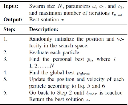
Fig 1: A standard particle swarm optimization (PSO) algorithm
Table 2: Examples representing particle i
Position j Position value Ranking of values Job order
1 -0.43 -2.98 3
2 3.14 -2.37 7
3 -2.98 -0.43 1
4 2.61 0.25 6
5 1.56 1.56 5
6 0.25 2.61 4
7 -2.37 3.14 2
Table 3: Position information examples obtained from the permutation solutions
Position j NEH/TS solution
Random value Mapping value
1 3 -3.14 -0.43
2 7 -2.37 3.14
3 1 -0.43 -2.98
4 6 1.56 2.61
5 5 0.25 1.56
6 4 2.61 0.25
7 2 -2.98 -2.37
where d is the dimension of the search area and tisthe iteration number. The position and velocity of particlei in iteration t
are 𝛸𝑖𝑡= 𝛸
𝑖,1𝑡 , 𝛸𝑖,2𝑡 , 𝛸𝑖,3𝑡 , … , 𝛸𝑖,𝑑𝑡 and
𝑉𝑖𝑡= 𝑉𝑖,1𝑡, 𝑉𝑖,2𝑡 , 𝑉𝑖,3𝑡, … , 𝑉𝑖,𝑑𝑡 , respectively. Personal best
𝑝𝑖𝑡= 𝑝𝑖,1𝑡 , 𝑝𝑖,2𝑡 , 𝑝𝑖,3𝑡 , … , 𝑝𝑖,𝑑𝑡 corresponds to particle i and is
the best fitness value so far during time period t. The global
best is respected so that
𝑝𝑔𝑏𝑒𝑠𝑡 ,𝑗𝑡 = 𝑝 𝑔𝑏𝑒𝑠𝑡 ,1
𝑡 , 𝑝
𝑔𝑏𝑒𝑠𝑡 ,2
𝑡 , 𝑝
𝑔𝑏𝑒𝑠𝑡 ,3
𝑡 , … , 𝑝
𝑔𝑏𝑒𝑠𝑡 ,𝑑𝑡 , which
indicates the best fitness solution found since initialization. Inertia weight ω is used for controlling the convergence speed, 𝑐1 is the acceleration weight cognitive element,𝑐2 is the
weight of the social parameter, and 𝑟1and 𝑟2 are random
numbers uniformly distributed in the area of [0,1]. The personal best update processing of particle iand the current best (global best) solution in the swarm is updated using the minimizing the object function f.
Figure 1 show the procedure for the standard PSO approach.
3.
THE PROPOSED ALGORITHM
This PRHPSO algorithm consists of two main phases during the PSO evolution, namely the pattern reduction operator phase and regeneration operator phase. This section introduces pattern reduction and the regeneration operator, which are adapted into the PSO-based algorithm for solving the permutation flow-shop scheduling problem (PFSP).
3.1
Particle Encoding
In the PSO algorithm, the particles fly through the solution space engaging in social behaviour. Encoding particles in the population for the PFSP is an important issue. In order to find a suitable direct mapping between the positions (dimensions) of particles and the job sequence, this paper employs a heuristic approach called smallest position value (SPV) [38], which is used for converting the continuous values into permutations of the job sequence. In short, each particle is represented by n continuous values. In the decoding process, these continuous values are transformed into a permutation of the job sequence by the SPV rule. Table 2 illustrates the process of decoding a particle using the SPV rule.
The second column denotes the position values of the particle. The fourth column indicates the increase of each value. According to the SPV value, -2.98 is the smallest position value. The first job order in 𝑥𝑖,1 is 3. Then, -2.37 is picked and
𝑥𝑖,2is assigned in 7. The remaining values are picked
according to their ranking to construct the permutation. Thus, the complete job permutation π = (3, 7,1,6,5,4,2).
3.2
Particle Initialization
To ensure that the initial swarm has a quality solution, the NEH [4] heuristic algorithm and TS [23] are applied to generating two solutions. The remaining particles are given random values (including position and velocity) using
𝑥𝑖,𝑗 = 𝑥𝑢,𝑏∗ 𝑟 (7)
𝑣𝑖,𝑗 = 𝑣𝑙,𝑏+ 𝑣𝑢,𝑏− 𝑣𝑙,𝑏 ∗ 𝑟 (8)
where 𝑥𝑢,𝑏 = 5.0, 𝑣𝑙,𝑏 = −5.0, 𝑣𝑢,𝑏 = 5.0, and r is in the
interval [0,1]. Table 3 shows an example of position values generated from the permutation results.
3.3
Pattern Reduction
In the first phase, the concept of the pattern reduction (PR) technique was presented by Chiang et al. [39]. It was used for solving a clustering problem. According to previous research, the PR can be used in meta-heuristics algorithms for solving the combinatorial optimization problem.
In this paper, we modify the basic PR for the PFSP. This operator is divided into two parts, namely detection and compression. The goal of PR is to quickly eliminate redundant process during PSO processing. Details of the two parts are given below. Before the PR phase, the current best solution will be called parent 1 and used in regeneration operator phases.
3.3.1
Detection operator:
In this operator, the solutions are inspected against all positions (dimensions), which are marked as either undetected or detected, (detected positions are indicated by 1, others by 0). The detection vector is defined as.
Table 4: Rearrangement the of permutationusing newposition value and spv rule
(Iteration i-1) Position j
Position value
Ranking of values
Job order
1 -0.43 -2.98 3
2 3.14 -2.37 7
3 -2.98 -0.43 1
4 2.61 0.25 6
5 1.56 1.56 5
6 0.25 2.61 4
7 -2.37 3.14 2
(Iteration i) Position j
Position value
Ranking of values
Job order
1 1.26 -2.01 4
2 -0.72 -1.67 7
3 1.68 -0.72 2
4 -2.01 0.53 5
5 0.53 1.26 1
6 3.91 1.68 3
[image:4.595.87.245.343.503.2]7 -1.67 3.91 6
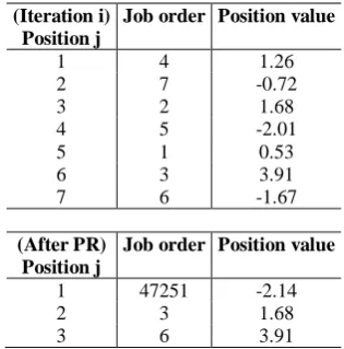
Table 5: Rearrangement of position values after the pattern reduction operator
(Iteration i) Position j
Job order Position value
1 4 1.26
2 7 -0.72
3 2 1.68
4 5 -2.01
5 1 0.53
6 3 3.91
7 6 -1.67
(After PR) Position j
Job order Position value
1 47251 -2.14
2 3 1.68
3 6 3.91
Table 1 shows that all of the five permutation solutions have three detected positions (1, 2, and 3), which have respective element values of {1}, {2}, and {3}. The following rules are used for determining the trigger condition for the compression operator.
i.) If there are fewer than two positions marked as detected.
ii.) If there are at least two positions labelled detected, but none is marked as connected.
iii.) If there are two or more elements marked as connected.
If the solutions belong to casei.) or case ii.), the compression part is not triggered.
3.3.2
Compression operator:
In this part, the connected positions can be readily obtained from common sub-solutions by interacting with the detection vector. If the connective sub-solutions detected are redundant, they can be merged into one element. Considering the previous example in this operator, elements {1}, {2}, and {3}
can be merged into one set {123}. The {123} may find the connective sub-solution {64} and the two sub-solutions may be combined into one set {12364}. Then the set {12364} will be compressed into one element {1}. Finally, the solution will become {157}, which means only the makespan of the job sequence {157} needs to be calculated, rather than {1236457}.
3.4
Particle Updating
A particle moves in a direction according to the inertia weight. The best position and the best position so far of other particles can be formalized using Eqs.5 and 6. These two equations are used for determining the final position of particle i in iteration t. However, new velocity and position values are obtained aftereachiteration. Thus, after updating particle position values, the permutation jobs sequence must be rearranged by the SPV rule. Table 4 shows how to determine the new permutation sequence after particle update. Table 5 shows another example of how to determine and reduce the dimensions of the new position values after the PR operator. It can be seen in Table 5 that the job sequence {4725136} will be reduced and compressed into the new job sequence {436}. Thus the PR can reduce the computation time.
After the PR operator, we can get the convergence solution, parent 2. Although the PR approach can reduce the computation time, it may cause particles to converge very quickly. Thus, the regeneration operator method is used for improving the quality and diversity of the PSO algorithm.
3.5
Regenerate Operator
The concept in this phase uses the crossover operator - order operator [40] (OX) to reconstruct all particles by using parent 1 and parent 2. The use of parent 1, parent 2 and (OX) operator should be used for reconstructing the remaining particles. Fig. 2 shows how the regeneration operator rebuilds the remaining particles. After the reconstruction phase, each new particle (solution) is used for reinitializing the position and velocity values according to the SPV rule. This new population will be evaluated by using the PSO algorithm until the termination criteria are reached, but without employing the PR operator again.
3.6
SA-based Local Search
In order to add diversity and improve quality, four neighborhood perturbation methods (SA-based VNS local search) can be used in the SA local search, namely pair-swap, insertion, inversion, and displacement.
a) Pair-Swap: Randomly select two distinct positions and swap them.
b) Insertion: Randomly select two distinct positions (a, b) and insert b in front of a.
c) Inversion: Invert the subsequence between two random positions in the solution.
Fig 2: Example regeneration operator.
Fig 3: Example of the perturbation methods.
3.7
The PRHPSO algorithm
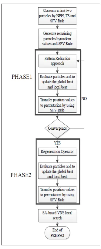
The PRHPSO algorithm is a two-phase hybrid PSO-based algorithm for solving PFSP. Phase 1 uses the PR technique to reduce computation time and, in phase 2, a regeneration operator is adopted to balance exploitation and exploration and restart the PSO evolution process without using the PR operator.
[image:5.595.54.277.381.586.2]Finally, the SA-based local search preserves the best solution after the regeneration operator.The PRHPSO algorithm is illustrated in Fig. 4.
Fig 4: The flowchart of the PRHPSO.
3.8
An Example
Considering the five solutions in Table 1, the process for executing PRHPSO for this example is shown in Fig. 5. The PR and regeneration operator are applied to the PSO convergence processing. Assuming that the current best solution sequence (parent 1) is {523641} before the PR operator, and parent 2 is {123456} at the PR operator, then parent 1 and parent 2 pass through the regeneration operator OX to reconstruct the remaining particles. Straightforward the PSO process, the best solution becomes {251364}. Finally, the best solution {251364} is adjusted to {314562} using the SA-based local search.
4.
EXPERIMENTAL RESULTS
Fig 5: An Example of PRHPSO algorithm.
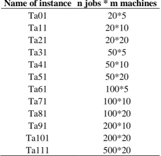
Table 6: The Taillard benchmarks for permutation flow-shop problem
Name of instance n jobs * m machines
Ta01 20*5
Ta11 20*10
Ta21 20*20
Ta31 50*5
Ta41 50*10
Ta51 50*20
Ta61 Ta71 Ta81 Ta91 Ta101 Ta111
[image:6.595.328.530.99.290.2]100*5 100*10 100*20 200*10 200*20 500*20
Table 7Parameter settings for permutation flow-shop instance
PSO parameters
Swarm size 50
# of iterations 1000 PR start iteration 20 # of simulations (R) 30
# of Regeneration Operator iterators
100
ω 0.9 to 0.4
𝑐1,𝑐2 2
SA parameters
Initial temperature T 100 Cooling coefficient β 0.99
TS parameters
[image:6.595.326.530.338.528.2]Size of Tabu list 7 # of iterations 1000
Table 8Experimental results of the PRHPSO against DPSO
Name of instance DPSO[28] PRHPSO
ARPD 𝑡𝑎𝑣𝑔 ARPD 𝑡𝑎𝑣𝑔
Ta01 0.94 0.40 0.06 0.78 Ta11 4.74 0.47 0.69 0.92 Ta21 4.13 0.63 0.52 0.73 Ta31 0.77 1.76 0.18 2.36 Ta41 6.15 1.88 2.80 2.65 Ta51 4.05 2.27 2.93 3.22 Ta61 0.33 6.23 0.04 5.94
Ta71 2.01 6.42 0.92 5.77
Ta81 3.72 7.27 2.08 6.29
Ta91 15.74 23.35 0.69 17.86
Ta101 3.01 25.68 2.21 21.03
Ta111 7.47 142.93 1.97 109.76
[image:6.595.88.246.381.534.2]Average 4.82 19.94 1.37 16.12
Table 9: Experimental results of the PRHPSO against PSOVNS
Name of instance DPSO[28] PRHPSO
ARPD 𝑡𝑎𝑣𝑔 ARPD 𝑡𝑎𝑣𝑔
Ta01 0.03 9.84 0.06 0.78
Ta11 0.04 13.93 0.69 0.92
Ta21 0.18 21.57 0.52 0.73
Ta31 0.02 22.37 0.18 2.36
Ta41 1.73 30.56 2.80 2.65
Ta51 2.12 46.80 2.93 3.22
Ta61 0.06 43.72 0.04 5.94
Ta71 0.45 59.43 0.92 5.77
Ta81 1.57 92.89 2.08 6.29
Ta91 0.76 121.70 0.69 17.86
Ta101 1.49 190.49 2.21 21.03
Ta111 1.17 522.22 1.97 109.76
Average 0.88 106.95 1.37 16.12
The dataset generated by Taillard [41] was used in this evaluation. The well-known benchmark composed of 120 instances from 20 jobs and 5 machines (Ta01) to 500 jobs and 20 machines (Ta111) for permutation flow-shop scheduling, as shown in Table VI. All experiments were performed on a computer with a core(TM)2 Quad Q9400 2.66GHz Intel CPU with 2GB of memory running on Microsoft Windows 7. In the experiments, all of the programs were implemented using Java language. The PSO, SA, and TS parameter settings are shown in Table VII. Table VIII and Table IX show a comparison of the simulation results. The average percentage relative deviation ARPD is shown in Eq. 10 and the average computation time is denoted as𝑡𝑎𝑣𝑔seconds.
ARPD = 𝑄𝑖−𝑄𝑏𝑘𝑠
𝑄𝑏𝑘𝑠 ∗ 100% /R 𝑅
𝑖 (10)
where 𝑄𝑖 denotes the values of the makespan of algorithm
found, 𝑄𝑏𝑘𝑠 indicates the best known solutions, and R denotes
[image:6.595.79.254.585.771.2]Table VIII and Table IX show the results of the DPSO, PSOVNS, and the proposed PRHPSO algorithms for the best known solutions for the Taillard’s benchmark. In Table VIII, the PRHPSO is slightly slower than the DPSO in the dataset Ta01 to Ta61. This is because the DPSO does not have the SPV-rule mapping and rearranging strategy. By using the SPV-rule, regeneration operator and SA-based local search, the PRHPSO outperforms the DPSO in ARPD measure. In Table IX, the PRHPSO is faster than the PSOVNS almost 6 times in total average; except in Ta61 and Ta91, it losses quality in ARPD. This is because the PR operator leads the PSO to fast convergence, and regeneration operator and SA increase the quality.
5.
CONCLUSIONS
A two-phase mememic PSO algorithm (PRHPSO) is proposed for solving the permutation flow-shop scheduling problem. The experimental results indicate that the proposed method is faster than other algorithms with regard to CPU time in large scale of benchmarks and has some quality loss compared to PSOVNS. Many things can be done to refine this algorithm. (1) More effective detection strategies should be developed for the pattern reduction phase of algorithm. (2) In making the ARPD solutions better than those of PSOVNS or other effective algorithms, another powerful regeneration approach should be considered, meaning to enhance the solution searching abilities of particles.
6.
ACKNOWLEDGMENTS
This work was supported in part by the National ScienceCouncil, Taiwan, R.O.C., under grants NSC 100-2218-E-006-
031-MY3.
7.
REFERENCES
[1] S. M. Johnson, “Optimal two- and three-stage production schedules withsetup times included,” Naval Research Logistics Quarterly, vol. 1, pp.61–68, 1954.
[2] A. H. G. Rinnooy Kan, Machine scheduling problems: Classification,complexity and computations. Martinus Nijhoff, The Hague, 1976.
[3] M. R. Garey, D. S. Johnson, and R. Sethi, “The complexity of flowshopand jobshop scheduling,” Mathematics of Operations Research, vol. 1,pp. 117– 129, 1976.
[4] M. Nawaz, E. E. Enscore Jr, and I. Ham, “A heuristic algorithm for them-machine, n-job flow-shop sequencing problem,” OMEGA, vol. 11,no. 1, pp. 91–95, 1983. [5] I. H. Osman and C. N. Potts, “Simulated annealing for
permutationflow-shop scheduling,” Omega, vol. 17, no. 6, pp. 551–557, 1989.
[6] C. Low, J. Yeh, and K. Huang., “A robust simulated annealing heuristicfor flow shop scheduling problem,” International Journal of AdvancedManufacturing Technology, vol. 23, pp. 762–767, 2004.
[7] E. Nowicki and C. Smutnicki, “A fast tabu search algorithm for thepermutation flow-shop problem,” European Journal of OperationalResearch, vol. 91, no. 1, pp. 160–175, 1996.
[8] J. P.Watson, L. Barbulescu, L. D. Whitley, and A. E. Howe, “Contrastingstructured and random permutation flow-shop scheduling problems:Search-space topology
and algorithm performance,” ORSA Journal onComputing, vol. 14, pp. 98–123, 2002.
[9] C. R. Reeves, “A genetic algorithm for flowshop sequencing,” Computersand Operations Research., vol. 22, pp. 5–13, January 1995.
[10]O. Etiler, B. Toklu, M. Atak, and J. Wilson., “A genetic algorithmfor flow shop scheduling problems,” The Journal of the OperationalResearch Society, vol. 55, no. 8, pp. 830–835, 2004.
[11]T. St¨utzle, F. Intellektik, F. Informatik, and T. H. Darmstadt, “Anant approach to the flow shop problem,” in In Proceedings of the6th European Congress on Intelligent Techniques & Soft Computing(EUFIT’98, 1997, pp. 1560–1564.
[12]C. Rajendran and H. Ziegler, “Ant-colony algorithms for permutationflowshop scheduling to minimize makespan/total flowtime of jobs,”European Journal of Operational Research, vol. 155, no. 2, pp. 426– 438,2004..
[13]Q.-K. Pan, M. F. Tasgetiren, and Y.-C. Liang, “A discrete differentialevolution algorithm for the permutation flowshop scheduling problem,”Computers and Industrial Engineering, vol. 55, no. 4, pp. 795– 816,2008.
[14]Q.-K. Pan, L. Wang, and B. Qian, “A novel differential evolution algorithmfor bi-criteria no-wait flow shop scheduling problems,” Computersand Operations Research, vol. 36, pp. 2498–2511, 2009.
[15]B. Qian, L. Wang, R. Hu, W.-L. Wang, D.-X. Huang, and X. Wang, “Ahybrid differential evolution method for permutation flow-shop scheduling,”The International Journal of Advanced Manufacturing Technology,vol. 38, pp. 757–777, 2008.
[16]Y. Zhang, X. Li, and Q. Wang, “Hybrid genetic algorithm for permutationflowshop scheduling problems with total flowtime minimization,”European Journal of Operational Research, vol. 196, no. 3, pp. 869–876,2009. [17]T.-C. Chiang, H.-C. Cheng, and L.-C. Fu, “NNMA: An effective memeticalgorithm for solving multiobjective permutation flow shop schedulingproblems,” Expert Systems with Applications, vol. 38, no. 5, pp. 5986 – 5999, 2011..
[18]S. Kirkpatrick, C. D. Gelatt, and M. P. Vecchi, “Optimization bysimulated annealing,” Science, vol. 220, pp. 671–680, 1983.
[19]N. Mladenovic, “Variable neighborhood search,” Computers and OperationsResearch, vol. 24, no. 11, pp. 1097–1100, 1997.
[20]E. Taillard, “Some efficient heuristic methods for the flow shop sequencingproblem,” European Journal of Operational Research, vol. 47, no. 1,pp. 65–74, Jul. 1990.
[21]T. Aldowaisan and A. Allahverdi, “New heuristics for no-wait flowshopsto minimize makespan,” Computers and Operations Research, vol. 30,no. 8, pp. 1219 – 1231, 2003.
shops,” Computers andOperations Research, vol. 35, pp. 3001–3008, 2008.
[23]F. Glover and M. Laguna, Tabu Search. Norwell, MA, USA: KluwerAcademic Publishers, 1997.
[24]N. Metropolis, A. W. Rosenbluth, M. N. Rosenbluth, A. H. Teller, andE. Teller, “Equation of State Calculations by Fast Computing Machines,”The Journal of Chemical Physics, vol. 21, no. 6, pp. 1087–1092, 1953.
[25]J. Kennedy and R. Eberhart, “Particle swarm optimization,” in NeuralNetworks, 1995. Proceedings., IEEE International Conference on, vol. 4,1995, pp. 1942–1948.
[26]J. Kennedy and R. C. Eberhart, “A discrete binary version of the particleswarm algorithm,” in IEEE International Conference on Systems, Man,and Cybernetics,, vol. 5, 1997, pp. 4104–4108.
[27]M. Tasgetiren, M. Sevkli, Y.-C. Liang, and G. Gencyilmaz, “Particleswarm optimization algorithm for permutation flowshop sequencingproblem,” in Ant Colony Optimization and Swarm Intelligence. SpringerBerlin / Heidelberg, 2004.
[28]K. Rameshkumar, R. Suresh, and K. Mohanasundaram, “Discrete particleswarm optimization (dpso) algorithm for permutation flowshopscheduling to minimize makespan,” in Advances in Natural Computation,ser. Lecture Notes in Computer Science. Springer Berlin /Heidelberg, 2005, vol. 3612, p. 572581.
[29]Z. Lian, X. Gu, and B. Jiao, “A similar particle swarm optimizationalgorithm for permutation flowshop scheduling to minimize makespan,”Applied Mathematics and Computation, vol. 175, pp. 773–785, 2006.
[30]C.-J. Liao, C.-T. Tseng, and P. Luarn, “A discrete version of particleswarm optimization for flowshop scheduling problems,” Computers andOperations Research, vol. 34, pp. 3099–3111, 2007.
[31]B. Liu, L. Wang, and Y.-H. Jin, “An effective pso-based memeticalgorithm for flow shop scheduling,” Systems, Man, and Cybernetics,Part B: Cybernetics, IEEE Transactions on, vol. 37, no. 1, pp. 18 –27,feb. 2007. [32]M. F. Tasgetiren, Y.-C. Liang, M. Sevkli, and G.
Gencyilmaz, “A particleswarm optimization algorithm
for makespan and total flowtime minimizationin the permutation flowshop sequencing problem,” EuropeanJournal of Operational Research, vol. 177, no. 3, pp. 1930 – 1947, 2007.
[33]C. Zhang, J. Sun, X. Zhu, and Q. Yang, “An improved particle swarmoptimization algorithm for flowshop scheduling problem,” InformationProcessing Letters, vol. 108, pp. 204–209, 2008.
[34]D. Sha and H. Hung Lin, “A particle swarm optimization for multiobjectiveflowshop scheduling,” The International Journal of AdvancedManufacturing Technology, vol. 45, pp. 749–758, 2009.
[35]C. Zhang, J. Ning, and D. Ouyang, “A hybrid alternate two phases particleswarm optimization algorithm for flow shop scheduling problem,”Computers and Industrial Engineering, vol. 58, pp. 1–11, February 2010.
[36]H. Liu, L. Gao, and Q. Pan, “A hybrid particle swarm optimization withestimation of distribution algorithm for solving permutation flowshopscheduling problem,” Expert Systems with Applications, vol. 38, pp.4348– 4360, 2011.
[37]Y. Shi and R. Eberhart, “A modified particle swarm optimizer,” in Proceedingsof IEEE international conference on evolutionary computation,1998, pp. 69– 73.
[38]J. C. Bean, “Genetic algorithms and random keys for sequencing andoptimization,” ORSA Journal on Computing, vol. 6, no. 2, pp. 154–160,1994.
[39]M.-C. Chiang, C.-W. Tsai, and C.-S. Yang, “A time-efficient patterreduction algorithm for k-means clustering,” Inf. Sci., vol. 181, no. 4,pp. 716–731, Feb. 2011.