Numerical Algorithms for Solving One Type of Singular Integro Differential Equation Containing Derivatives of the Time Delay States

http://dx.doi.org/10.4236/am.2015.68123

How to cite this paper: Chiang, S. and Herdman, T.L. (2015) Numerical Algorithms for Solving One Type of Singular Inte-gro-Differential Equation Containing Derivatives of the Time Delay States. Applied Mathematics, 6, 1294-1301.

http://dx.doi.org/10.4236/am.2015.68123

Numerical Algorithms for Solving One Type

of Singular Integro-Differential Equation

Containing Derivatives of the

Time Delay States

Shihchung Chiang

1*

, Terry L. Herdman

2

1_{Department of Finance, Chung Hua University, Hsinchu, Taiwan} 2_{Department of Mathematics, Virginia Tech, Blacksburg, VA, USA} Email: *_{[email protected], [email protected]}

Received 18 June 2015; accepted 20 July 2015; published 24 July 2015

Copyright © 2015 by authors and Scientific Research Publishing Inc.

This work is licensed under the Creative Commons Attribution International License (CC BY). http://creativecommons.org/licenses/by/4.0/

Abstract

This study presents numerical algorithms for solving a class of equations that partly consists of derivatives of the unknown state at previous certain times, as well as an integro-differential term containing a weakly singular kernel. These equations are types of integro-differential equation of the second kind and were originally obtained from an aeroelasticity problem. One of the main contributions of this study is to propose numerical algorithms that do not involve transforming the original equation into the corresponding Volterra equation, but still enable the numerical so-lution of the original equation to be determined. The feasibility of the proposed numerical algo-rithm is demonstrated by applying examples in measuring the maximum errors with exact solu-tions at every computed nodes and calculating the corresponding numerical rates of convergence thereafter.

Keywords

Integro-Differential Equation of the Second Kind, Weakly Singular Kernel, Numerical Algorithms, Rates of Convergence

1. Introduction

was introduced by Burns, Cliff, and Herdman [1] in 1983. The system contains a form of linear singular inte-gro-differential equations with integration over a deterministic interval (i.e., equations not of the Volterra types). Other studies [2] [3] have presented the well-posedness of the problem regarding specific product spaces and the exact solutions of the original class of integro-differential equations of the first kind, and have reported numeri-cal methods and corresponding numerinumeri-cal results [4] [5]. Associated optimal control problems are topics dis-cussed in [6]. Another study [7] applied semigroup theory to this particular type of equation and constructed an associated abstract Cauchy problem. The current study presents a numerical algorithm for solving the type of equations containing not only the original aeroelastic integro-differential term as a part of the equation but also time-derivative states evaluated at different previous times. This new linear equation is in the category of “inte-gro-differential equations of the second kind”. The main purpose of this study is to develop feasible numerical algorithms for solving this type of integro-differential equation. According to previous studies (for example, [8]), all existing numerical methods can be used for solving only integro-differential equations of the second kind that can be transformed into Volterra integral equations of the second kind that linearly containing the state, and no numerical method (except the papers by current authors) has been proposed for solving the integro-differential equations of the second kind directly and the integro-differential equations of the second kind containing time delay states. The remainder of this paper is organized as follows: Section 2 presents the derivation of the asso-ciated Volterra integral equations of the second kind. Section 3 presents numerical algorithms used for directly solving singular integro-differential equations of the second kind. Section 4 presents the numerical results of test examples obtained by applying the numerical method described in Section 3. Finally, Section 5 presents a sum-mary of this study.

2. Problem Description

Consider the class of an integro-differential equation of the second kind expressed as follows:

(

)

1

( )

1

d

, d

l

i i l t

i

a x t a Dx f t

t

σ +

=

− + =

∑

 (1)

and the initial condition

( )

( )

, 0,

x s =φ s s≤ (2) where a a₁, ₂,,al+₁ are constants and σi, i=1,, ,l are nonnegative constants. The term x t

(

−σi

)

is the derivative of the delay state with respect to t, and the difference operator D is defined as

( ) ( )

0

d

t t

b

Dx g s x s s

−

=

_∫

.

The second part of the integrand represents

( )

(

)

t

x s =x t+s , and the first part is a weakly singular function

( )

1

[

, 0

]

g s ∈L −b ,

that is integrable, positive, nondecreasing, and weakly singular at s=0. Assume the forcing term f t

( )

is lo-cally integrable for t>0. Although a more general kernel g is also suitable, this study focuses on the Abel- type kernel and considers g s

( )

= s−p and s∈ −

[

b, 0

]

for 0< <p 1. A specific value of p=0.5 corres-ponds to the original aeroelastic problem. Assume that the initial condition φ

( )

s , for − ≤ ≤b s 0, is in L_1,g space, a weighted L₁ space with weight g

( )

⋅ .

If the differential part of the integro-differential term can be removed, that is, the term Dx₀ exists, then ap-plying the integration to Equation (1) forms a new equation of the following form:

(

)

1

(

)

1 0

( )

1 1 0

d , for 0 . t

l l

i i l t i i l

i i

a x t σ a Dx₊ aφ σ a Dx₊ f τ τ t b

= =

− + = − + + < ≤

∑

∑

∫

(

)

0 d p t b

Dx s− x t s s

−

=

_∫

+

is absolutely continuous with respect to t>0, and the product of the kernel and initial functions, g

( ) ( )

⋅ φ ⋅ , belongs to L₁

[

−b, 0

]

. Therefore, the corresponding weakly singular Volterra integral equation of the second kind is

(

)

( )

(

)

( )

( )

( )

1 1 0 0 0 1 1 1 0 d

d d d , for 0 .

t l

p

i i l

i

t l

p p

i i l l

i b t b

a x t a s t x s s

a f s s a s s s a s t s s t b

σ

φ σ φ φ

− + = − − + + = − − − + −

= − + + − − < ≤

∑

∫

∑

∫

∫

∫

3. Numerical Algorithms

The proposed algorithms involve using the separating variables method to directly solve the numerical solution of Equations (1) and (2). Without loss of generality, assume that b=1 and a₁=a₂ ==al+₁=1, the equation is expressed as

(

)

0

(

)

( )

( )

1 1

d

d , 0, 0,1 ,

d

l

p i

i

x t s x t s s f t t p

t

σ −

= −

− + + = > ∈

∑



∫

(3)

with initial data

( )

( )

, 0,

x s =φ s s≤ (4) where f t

( )

, t>0 is a locally integrable function.

Let σ =max

{

σ σ₁, ₂,,σ_l

}

, then Equation (3) can be divided into two categories: 0≤ ≤σ 1, and σ >1.

3.1.

0

≤ ≤

σ

1

For this category, following study [6], define a new functional ξ such that

( )

t s, x t

(

s

)

, 1 s 0,t 0.

ξ = + − ≤ ≤ > (5) Reformulate Equation (3) as a first-order hyperbolic partial differential equation

( )

t s,

( )

t s, , 1 s 0,

tξ sξ

∂ ₌ ∂ _{− ≤ ≤}

∂ ∂ (6) with the condition

(

)

0

( )

( )

1 1

, , d .

l

p i

i

t s t s s f t

tξ σ sξ

−

= −

∂ ∂

− + =

∂ ∂

∑

∫

(7)

Next, assume that the solutions to Equations (6) and (7) have the form

( )

( ) ( )

0 , n j j j

t s t B s

ξ α

=

=

∑

, (8)

where the bases, B_j

( )

s , j=0,, ,n are

( )

(

)

(

)

1 1 1 1 1 1 , , , 1 , , , 0, otherwise.

j j j

j

j j j j

j

s s

B s s s

τ τ τ

δ

τ τ τ

Specifically, B_j

( )

s and j=0,1,, ,n are piecewise linear functions. The mesh points, τ τ₀, ,₁,τn, are defined by − =1 τn<τn−₁<< <τ₁ τ₀=0 and δj=τj−1−τj>0, for j=1,, .n One restriction for the mesh points is

{

σ

₁,,

σ

l

}

⊂

{

τ τ

₀ , ₁,,

τ

n

}

, namely, the time lag terms coincide with some of the absolute values of mesh points.

After substituting the form of ξ previously defined in Equation (8) into Equations (6) and (7), the governing equations for α_j

( )

t and j=0,, ,n become the following equations:

( )

(

1

( )

( )

)

d 1

, 1, , ,

d j j j j

t t t j n

tα =δ α − −α = 

(9) and

( ) (

)

0

( )

( )

( )

1 0 1 0

d d

d .

d d

l n n

p

j j i j j

i j j

t B s t B s s f t

tα σ α s

−

= = − =

− + =

∑∑

∫

∑

(10)

By the property of the bases, rewrite Equation (10) as

( )

0

( )

( )

( )

1 1 0

d d

d ,

d i d

l n

p

j j

i j

t s t B s s f t

tασ α s

−

= − =

+ =

∑

∫

∑

(11)

where

( )

i t

σ

α are the corresponding terms of α_j

( )

t with respect to σ_i, i=1,, .l Define

1

d , 1, , ,

j

j p j

g s s j n

τ τ

− −

=

_∫

= 

and Equations (9) and (11) thus become

( )

(

1

( )

( )

)

d 1

, 1, , ,

d j j j j

t t t j n

tα =δ α − −α =  (12) and

( )

( )

(

1

)

(

1

( )

( )

)

( )

1 1 1 . i i i l n j j j

i j j

g

t t t t f t

σ σ

σ

α α α α

δ − δ −

= =

− + − =

∑

∑

(13)

This produces the following linear system of first-order ordinary differential equations:

( )

( )

( )

d

dtX t =AX t +G t , (14) where

( )

( )

( )

( )

T

0 1 n ,

X t = _

α

t

α

t 

α

t _

( ) ( )

1 1

2 2

1 1

1 1

0 0 0

1 1

0 0 0 ,

1 1

0 0 0

n n n n A

δ δ

δ δ

δ δ _{+ × +}

∗ ∗ ∗ ∗      ₋       ₋  =_{ }       −               

The procedure for obtaining the initial condition αi

( )

0 ,i=0,1,, ,n for the first-order ordinary differential system (14) is described as follows: For the initial condition, combine Equations (4), (5), and (8), and fix t=0; the state thus becomes

( )

( ) ( )

( )

0

0 , for 1 0.

n

i i i

x s α B s φ s s

=

=

∑

= − ≤ ≤

The structure of B₀

( ) ( )

s ,B s₁ ,, and B_n

( )

s indicates that α_i

( )

0 is equal to φ τ

( )

_i for i=0,1,, .n Next, to determine α₀

( ) ( )

t ,α₁ t ,,α_n

( )

t , apply an ordinary differential equation solver (Matlab “ode45”) to the system (14). Two methods can be used to solve x t

( )

, 0≤ ≤t 1, depending on the setting of variables: fix t=1 or s=0 in Equation (8). According to the property B_j

( )

s =1 at s=τ_j,j=0,1,, ,n the two choices become two cases for the solutionx t

( )

, 0≤ ≤t 1:

Case 1:

(

)

( ) ( )

( )

0

1 1 1 ,

n

i j j i i

j

x τ α B τ α

=

+ =

∑

=

and Case 2:

(

)

(

) ( )

0

(

)

0

1 1 0 1 .

n

i j i j i

j

x τ α τ B α τ

=

+ =

∑

+ = +

In Case 1, solve for α_i

( )

t ,i=0,1,, ,n based on Equation (14) and set t=1. Thus, α_i

( )

1 yields the corresponding solutions x

(

1+τ_i

)

,i=0,1,, .n In Case 2, solve for α₀

( )

t by using Equation (14).

Subsequently, set t= +1 τi to obtain α0

(

1+τi

)

for i=0,1,, .n Therefore, α0

(

1+τi

)

is the solution

(

1 i

)

x +τ for i=0,1,, .n

A similar procedure can be extended to solve x t

( )

, for 1< < ∞t .

3.2.

σ

>

1

For this category, Equation (3) can be rewritten as

(

)

0

(

)

1

(

)

( )

1

(

)

1 1

d d

d d d ,

d d

l

p p p

i i

x t s x t s s s x t s s f t s x t s s

t _σ t _σ

σ

− − − − −

= − − −

   

− + _ + + + _= + _ + _

   

∑



∫

∫

∫

then it becomes

(

)

0

(

)

( )

1

(

)

1

d d

d d ,

d d

l

p p

i i

x t s x t s s f t s t s s

t σ t σ

σ − − − φ

= − −

 

− + + = + _ + _

 

∑



∫

∫

a similar form of Equation (3) except for the integral interval of the second term on the left hand side, but this new equation can be treated by reconsidering the discretization interval to be

[

−σ, 0

]

; namely, by resetting the mesh points as − =σ τn <τn−₁ << <τ₁ τ₀ =0, and then follow the procedures introduced in Section 3.1.

4. Numerical Examples

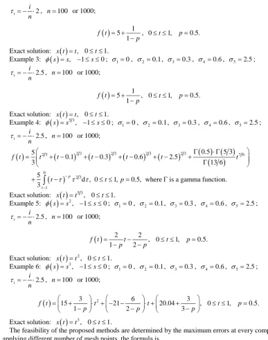
Consider examples involving p=0.5, initial conditions φ

( )

s , − ≤ ≤1 s 0, and forcing terms

( )

f t , for 0≤ ≤t 1.

Example 1: φ

( )

s =s2, − ≤ ≤1 s 0; σ =₁ 0, σ =₂ 0.1, σ =₃ 0.3, σ =₄ 0.6, σ =₅ 0.8, σ =₆ 0.9; i

i

n

τ = − , n=100 or 1000;

( )

2 2

12 5.4 ,

1 2

f t t t

p p

= ⋅ − + −

− − 0≤ ≤t 1, p=0.5. Exact solution: x t

( )

=t2, 0≤ ≤t 1.

2 i

i

n

τ = − ⋅ , n=100 or 1000;

( )

1

5 1 f t

p = +

− , 0≤ ≤t 1, p=0.5. Exact solution: x t

( )

=t, 0≤ ≤t 1.

Example 3: φ

( )

s =s, − ≤ ≤1 s 0; σ =₁ 0, σ =₂ 0.1, σ =₃ 0.3, σ =₄ 0.6, σ =₅ 2.5; 2.5

i i n

τ = − ⋅ , n=100 or 1000;

( )

1

5 ,

1 f t

p = +

− 0≤ ≤t 1, p=0.5. Exact solution: x t

( )

=t, 0≤ ≤t 1.

Example 4: φ

( )

s =s5 3, − ≤ ≤1 s 0; σ =₁ 0, σ =₂ 0.1, σ =₃ 0.3, σ =₄ 0.6, σ =₅ 2.5; 2.5

i i

n

τ = − ⋅ , n=100 or 1000;

( )

(

)

(

)

(

)

(

)

( ) ( )

₍

₎

(

)

2 3 2 3 2 3 2 3

2 3 7 6

0

2 3

1

0.5 5 3

5

0.1 0.3 0.6 2.5

3 13 6

5

d , 0 1, 0.5, where is a gamma function. 3

p

t

f t t t t t t t

t τ − τ τ t p

−

 Γ ⋅Γ 

= _ + − + − + − + − + _

Γ

 

+

_∫

− ≤ ≤ = Γ

Exact solution:

( )

5 3

,

x t =t 0≤ ≤t 1. Example 5:

( )

2

, s s

φ = − ≤ ≤1 s 0; σ =₁ 0, σ =₂ 0.1, σ =₃ 0.3, σ =₄ 0.6, σ =₅ 2.5; 2.5

i i n

τ = − ⋅ , n=100 or 1000;

( )

2 2

,

1 2

f t t

p p

= −

− − 0≤ ≤t 1, p=0.5. Exact solution:

( )

2

,

x t =t 0≤ ≤t 1. Example 6:

( )

3

, s s

φ = − ≤ ≤1 s 0; σ =₁ 0, σ =₂ 0.1, σ =₃ 0.3, σ =₄ 0.6, σ =₅ 2.5; 2.5

i i n

τ = − ⋅ , n=100 or 1000;

( )

3 2 6 3

15 21 20.04 ,

1 2 3

f t t t

p p p

     

=_ + _⋅ + − −_{ }⋅ +_ + _

− − −

      0≤ ≤t 1, p=0.5.

Exact solution: x t

( )

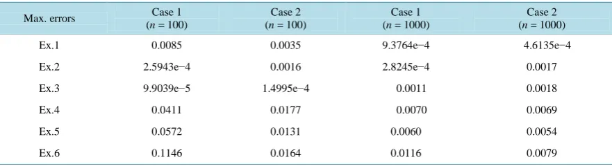
=t3, 0≤ ≤t 1.

The feasibility of the proposed methods are determined by the maximum errors at every computed nodes after applying different number of mesh points, the formula is

( )

Max error=max

α

i−x ti ,

for i=1, 2,, ;n n is the number of mesh points. α_i is the computed solution and x t

( )

_i is the exact solu-tion. The rate of convergence γ is defined as

( )

1

j x tj C n

γ

[image:6.595.83.471.83.575.2]

α − _{= ⋅ }    , for j= ∗1 k, 2∗k,, ;n k is a positive integer.

Table 1 and Table 2 contain the maximum errors at every computed nodes and mean rates of convergence

[image:7.595.93.534.100.220.2]

Table 1.The maximum errors at every computed nodes for the examples.

Max. errors Case 1

(n = 100)

Case 2 (n = 100)

Case 1 (n = 1000)

Case 2 (n = 1000)

Ex.1 0.0085 0.0035 9.3764e−4 4.6135e−4

Ex.2 2.5943e−4 0.0016 2.8245e−4 0.0017

Ex.3 9.9039e−5 1.4995e−4 0.0011 0.0018

Ex.4 0.0411 0.0177 0.0070 0.0069

Ex.5 0.0572 0.0131 0.0060 0.0054

[image:7.595.88.537.249.364.2]

Ex.6 0.1146 0.0164 0.0116 0.0079

Table 2.Mean rates of convergence evaluated at t=0.1,0.2,,1 for the examples.

Mean rates of convergence Case 1 (n = 100, 1000) Case 2 (n = 100, 1000)

Ex.1 1.1202 1.1514

Ex.2 −0.0886 0.3382

Ex.3 1.0315 −0.9663

Ex.4 0.9315 0.8200

Ex.5 1.0109 1.4067

Ex.6 0.9712 1.0185

have some vibration phenomena, the maximum errors in Table 1 provide sufficient evidence for the correctness of the numerical solutions.

Remark

This study presents a numerical method for directly solving the integro-differential equations of the second kind. The method involves discretizing the space s, and retains the variable t. The unknown states x t

( )

are repre- sented by α_i

( )

t ,i=0,1,, .n To solve system (14), which is a semi-discretized scheme, the authors suggest using an ordinary differential equation solver. The (mean) rates of convergence can be determined, although it depends on the separating variable form of the state as well as on the accuracy of the ordinary differential equa-tion solver applied (shown in the coming papers). Another approach to determining the rate of convergence in this observed study is to discretize both variables s and t, and this process results in a full-discretized scheme, as described in [3].

5. Summary

This study presents a numerical method for solving a class of singular integro-differential equations of the second kind that contain derivatives of the states at previous certain times of the finite history interval, as well as an integro-differential term containing a weakly singular kernel. The proposed equations can be transformed into Volterra integral equations of the second kind if the integro-differential term is integrable. This study presents direct numerical methods to the proposed equation. The tables of corresponding maximum errors and the mean rates of convergence show the feasibility of using the proposed numerical method for the equations.

References

[1] Burns, J.A., Cliff, E.M. and Herdman, T.L. (1983) A State-Space Model for an Aeroelastic System. Proceedings:22nd

IEEEConference on Decision and Control, San Antonio, December 1983, 1074-1077.

http://dx.doi.org/10.1109/CDC.1983.269685

[3] Herdman, T.L. and Turi, J. (1991) An Application of Finite Hilbert Transforms in the Derivation of a State Space Model for an Aeroelastic System. Journal of Integral Equations and Applications, 3, 271-287.

http://dx.doi.org/10.1216/jiea/1181075618

[4] Herdman, T.L. and Turi, J. (1991) On the Solutions of a Class of Integral Equations Arising in Unsteady Aerodynam-ics. In: Elaydi, S., Ed., Differential Equations: Stability and Control, Department of Mathematics, Trinity University, San Antonio, Texas, 241-248.

[5] Kappel, F. and Zhang, K.P. (1986) Equivalence of Functional Equations of Neutral Type and Abstract Cauchy Prob-lems. Monatshefte für Mathematik, 101, 115-133. http://dx.doi.org/10.1007/BF01298925

[6] Chiang, S. and Herdman, T.L. (2013) Revised Numerical Methods on the Optimal Control Problem for a Class of Sin-gular Integro-Differential Equations. Mathematics in Engineering, Science and Aerospace, 4, 176-189.

[7] Ito, K. and Turi, J. (1991) Numerical Methods for a Class of Singular Integro-Differential Equations Based on Semi-group Approximation. SIAM Journal on Numerical Analysis, 28, 1698-1722. http://dx.doi.org/10.1137/0728085 [8] Lubich, Ch. (1985) Fractional Linear Multistep Methods for Abel-Volterra Integral Equations of the Second Kind.