Multilayer Feed-Forward Neural Network Integrated with
Dynamic Learning Algorithm by Pruning of Nodes and
Connections
SiddhalingUrolagin, PhD.
Department of Computer Sc. and Engg.,
Manipal Institute of Technology,
Manipal-576104, Karnataka India.
ABSTRACT
Neural networks have found many applications in the real world. One of the important issues while designing the neural network is the size of the architecture. Dynamic learning algorithms aim to determine appropriate size of the network during learning phase. The dynamic learning algorithm by pruning involves in removing networks elements such as nodes, weights or biases from the network to reduce its size and make network size appropriate to solve a problem. In this paper two dynamic learning by pruning methods have been integrated with multilayer feed-forward neural network. The Optimal Brain Damage method is the connections (weights or biases) pruning method and Bottom Up Freezing method involves in freezing and pruning of nodes. The experiments have been conducted on MNIST handwritten database. The learning behavior of the multilayer feed-forward neural network integrated with OBD and BUF method has been analyzed.
Keywords
Pruning, Dynamic Learning, Freezing, Neural Network.
1. INTRODUCTION
Despite many advances, for neural networks to find general applicability in real-world problems, several questions need to be answered. One such open question is determining the most appropriate network size for solving a given problem [1]. If the network is too small then network does not learn at all [2]. The network does not have the required parameters so that it can learn according to the patterns and their classification. On other hand, if the network is too big then excessive number of hidden neurons may cause a problem called over fitting. The network will have so much information processing capability that it will learn insignificant aspects of training set, that are irrelevant to the general population [3] and it cannot generalize well. For a network to be able to generalize, it should have fewer parameters than there are data points in training set [4-6]. Hence the network should have a topology that is large enough to learn the mapping and at the same time small enough to generalize well. Until now selecting a topology is an art, which involves trying different topologies and choosing one that best satisfies the requirements. However,to overcome this time consuming approach,researchers have investigated the alternative approaches to conventional trial-and-error scheme and have
proposed dynamic learning algorithms to automate the process of neural network design. Dynamic learning algorithms are aimed at finding an adequate sized network for a given problem.The dynamic learning by pruning algorithms involve in the use of larger network architecture at the beginning and pruning it down to near optimum size as training progresses. Examples include Optimal Brain Damage (OBD) [7], optimal brain surgeon [8], interactive pruning [1,9], skeletonization [10] and Bottom Up Freezing (BUF) [11]. A good review on pruning algorithms has been covered in [2].Pruning of neural network has found several applications. In [12] the pruning is used for designing the neural network for hydrological prediction. It is shown in [12] that the quality of forecast is improved because of pruning of less influential parameters. The application of neural network pruning for sonar image recognition has been described in [13]. The synthesizing of desired filter using multilayer neural network along with pruning algorithm is presented in [14]. This research work focuses on integrating pruning algorithms with multilayer feed-forward neural network and apply it for handwritten numeral recognition. In section 2 details about the dynamic learning by pruning methods has been given. In this paper two known pruning methods have been selected and they are OBD of [7] and BUF of [11]. The OBD involves in identifying least significant parameters from the network and prune them during the training period. The BUF algorithm has two phases: local freezing and node pruning. When contribution of a node falls below a certain threshold it is frozen and when a node is frozen more oftenly then it is pruned permanently from the network. Both these methods have been further elaborated in section 3 and 4 respectively. The neural networks have been integrated with these dynamic learning methods separately and learning behavior has been analyzed.The details about database and feature extraction method used in this research areexplained in section 5. In section 6 experiments conducted and analysis of results are covered. Finally the conclusion is given in section 7.
2. DYNAMIC LEARNING BY PRUNING
METHODS
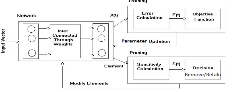
Fig. 1: Neural network training process. Network. As shown Fig. 1 the network consists of a number
of layers. A layer intern consists a number of nodes. In a typical multilayer feed-forward neural network, nodes of lower layer are connected to nodes of higher layer through weights.
Let
wij
denotes the weight between connectionsnode j
tonodei
. On a particular input vector at time t let Xˆ(t) isvector denoting the desired output of neural network. The actual output vector X(t) of the network which may differ from vectorXˆ(t). Forward calculation for
nodei
is:j
x
j
ij
w
i
a
and
)
i
f(a
i
x
(1)
Where, f is transfer function,
x
iis output ofnodei
.Thedifference between actual output X(t) produced by the neural network and output expected
X
ˆ
(t)
is usually calculated as summation of square error E(t).)
i
xˆ
i
(x
2
n
1
i
E(t)
2
1
(2)
Where n number of nodes at output layer. The aim of the learning procedure as shown in Fig.1 is to adjust weights and
biases such that error E(t) will be minimized. A brute force parameter pruning method could be to set every parameter to zero and evaluate change in E(t). If it increases then restore the parameter value otherwise remove it [2]. However the brute force method is not an effective method for parameter elimination. There are two most popular pruning methods are found in the literature: sensitivity based pruning and penalty term based pruning. The sensitivity based pruning method can be represented as shown in Fig. 2. The sensitivity based pruning methods estimate the sensitivity S(t) of the error E(t) to removal of a parameter. During training process the sensitivity of all the parameters of the network are calculated. The parameters with least sensitivityS(t) will be removed[1] form the network and network is retrained. This process is usually repeated several times.
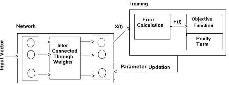
The penalty term pruning method is represented in Fig. 3. In these methods the forward calculation and backward propagation is same as that of standard learning method. However penalty terms are added with objective function that rewards the network for choosing efficient solution. The penalty term methods modify the cost function so that while parameter modification the function drives unnecessary parameters to zero and in effect removes them during training.
[image:2.595.100.502.552.710.2]Fig. 3: Neural network pruning by penalty term method.
3. OPTIMAL BRAIN DAMAGE
The Optimal Brain Damage (OBD) pruning method involves in selectively deleting the parameters to reduce the size of the network. This process of selectively deleting the parameters is carried out during the training process. In the OBD a method to measure the saliency of a parameter based on the objective function is derived. The saliency of a parameter is considered as change in the objective function caused by deleting that parameter. The OBD technique uses the second order derivative of the objective function with respect to the parameters to compute the saliencies.Here object function is defined as approximation of error E by Taylor series. A perturbation δU of the parameter vector will change the object function by
)
δu
3
O(
u j
δ
ui
δ
j
i
hij
2
1
u2
i
δ
i
hii
2
1
ui
δ
i
gi
δE
(3)Where,
ui
can control one or more connectionswij
or biasesi
b
,U
is a vector ofui
,δ
ui
is perturbation inui
,g
i
iscomponent of gradient GofEwith respect to
U
,h ij
are elements of Hessian matrix H of E with respect toU
u j
ui
E2
hij
and
ui
E
gi
(4)
The goal is to find a set of parameters whose deletion will cause the least increase of E. Toevaluate
δE
,several approximations are made. Extremal Approximation: the extremal approximation assumes that the parameter deletion will be performed after training has converged. The parameter vector is then at a (local) minima of E and first term in the equation can be neglected. Furthermore, at local minimum, all thehii
’s are non-negative, so any perturbation of parameter will cause E to increase or stay the same; DiagonalApproximation: the diagonal approximation assumes that the
δE
caused by deleting several parameters is the sum of theδE
’s caused by deleting each parameter individually, so third term in the equation discarded;Quadration approximation: the quadration approximation assumes that the cost function is nearly quadratic, so that the last term is the equation can be neglected.By simplifications (3) reduced to term containing perturbation in saliency and diagonal element of Hessian matrix.u
2
i
δ
i
hii
2
1
δE
(5)
Now we need an efficient way of computing the diagonal second derivatives
h
ii
. Such a procedure was derived in [15] and was the basis of a back-propagation method used extensively in various applications. Here the objective function is taken as Mean Squared Error (MSE). In a shared-weight network, a single parameteru
k
can control one or more connections:k
u
ij
w
for all ,(i,j)Vk, where Vkis a set of index pairs. By the chain rule, the diagonal terms of H are given by
2 ij w E 2 k V j) (i, kk h
(6) The summand can be expanded as:2
j
x
2
i
a
E
2
2
ij
w
E
2
(7)The second derivatives are back propagated from layer to layer:
i
x
E
)
i
(a
f
2
l
a
E
2
l
2
li
w
2
)
i
(a
f
2
i
a
E
2
(8))
i
(a
f
)
i
x
i
2(a
2
)
i
(a
f
2
2
i
a
E
2
(9)for all units i in the output layer.In some cases, the second term of the right hand side of the last two (8) and (9) equations (involving the second derivative of f) can be neglected.
4. BOTTOM-UP FREEZING
ALGORITHM
In recent years, many neural networks algorithms have been proposed by researchers to overcome the inefficiency of ANNs with predetermined architecture. They all address ANNs with dynamic structures where the learning algorithms not only search the weights space, but also modify the architecture of the network during the training. Here an investigationof Bottom-Up Freezing (BUF) algorithm based [11] is made, which alters nodes and ultimately optimizes the network architecture as learning proceeds. The basic idea underlying the BUF algorithm is to evaluate the hidden nodes and isolate (freeze) those hidden nodes whose contribution to the convergence of the network falls below a certain threshold. When a node is frozen, it will not participate in the training process for a certain period of time or for a given number of training examples and this is called as local pruning. When the freezing period of a node is over, it is returned to the network. The state of the node at the time of return will be the same as its state at the time of freezing. If a node freezes very often and the number of instances that a node was frozen exceeds a certain limit, the node is permanently removed from the network i.e. pruning of the node. The pruning occurs when a node is found to be redundant and ineffective to the progress of learning a problem. The local freezing and node pruning of the BUF approach allows a network to change its underlying structure and adapt dynamically to the ever-changing problem space as the training proceeds.
4.1 Local Freezing
In the local freezing the error signal e(t) of node i in the layer l is measured as given in (10) over a single training pattern presented at t time. Then e(t) can be used to evaluate the contribution of node i to the network convergence.
2
)
ij
w
i
(Δ
(t)
l
i
e
(10)
Where
ij
w
represents the outgoing weight of node i.Let
λS
ρ represent an
ρ
approximation, where Srepresent the size of the training set andλ
is set by the user. A node is a candidate for local freezing if its error signal did not decrease in the last ρ consecutive presentations of the training examples. The rate of increase of error signale(t) is computed as error rate, which is,100
1)
1)
e(t
e(t)
(
(t)
l
i
γ
(11)
The freezing time of a node (i.e., the number of presentations that a node does not participate in the training process) is
decided using the distribution of the errors of
ρ
consecutive increases in the error signals, which is calculated as,] l i μ[γ ρ ] l i μ[γ (t) l i γ ρ 1 t l i D
(12)Where
μ[
.
]
represents the mean.The magnitude ofl
i
D
shows the degree of poor behavior of node iduring the
ρ
consecutive presentations of the training examples.The magnitude of Dis used as the freezing time; thus, a larger Dmeans a longer freezing time. Freezing the insignificant nodes during the training process will speed up the convergence.4.2 Relative Importance of a Node
The number of times a node has been frozen, m is used to approximate the relative importance of that node to the convergence of a network. The magnitude of mis a clear indication of the contribution of a node to reducing the errorE(t). The relative importance, R, of a given node is defined as follows:
otherwise
m
2
frozen
is
l
i
node
if
m
2
1)
(m
2
l
i
R
(13)The relative importance of a node is a decreasing function based on the magnitude of m. At the beginning of the training process it is set to the value 2. The relative importance of a set of nodes is represented by the vector
R
. As the training proceeds, the number of frozen nodes as well as the number of times that a given node is frozen increases. Similarly, the variance ofR
,σ
[
R
]
2
, increases, whereas the mean of the values of
R
,μ[R]
, decreases. One of the key questions in the pruning algorithm is when is the proper time to remove a node from the network architecture. In BUF, the basic idea underlying the node removal is to analyze the freezing behavior of a hidden node and remove the node if it freezes very frequently. A node that freezes frequently is referred as node trashing.4.3 Node Pruning
Let's assume that during the training of a network a node is frozen relatively large number of times. If this node freezes one more time as the learning progresses, due to a small change in the magnitude of R(relative importance) of this node, the variance and the mean of relative importance of all nodes,
R
of the network do not change significantly. However when the difference between consecutive meanΔμ
and varianceΔσ2 of relative importance of all the nodes is inspected, it is seen that magnitude of minimum values of allμ
decreases. The
μ
and
σ
2of a node i in layer l are computed as,
1)]
(t
l
i
μ[R
(t)]
l
i
μ[R
Δμ
1)]
-(t
l
i
[R
2
σ
(t)]
l
i
[R
2
σ
2
σ
Thus, we can define the pruning time of a node as the time when the min [Δμ] changes (reduces). However, this criterion is not suitable at the beginning of the training process when freezing frequency of a node is not high and a single freeze reduces the value of min[Δμ]. To solve this problem, in addition to inspecting the value of min[Δμ] we also use the consecutive delta variances, Δσ2to determine a freezing candidate.At the beginning of a training process, a single freezing of a node changes the magnitude of its Rby a relatively large factor. Therefore, the differences between consecutive variances are high. However, as the learning progresses and a node show ill behavior and its mgets larger, further freezing of such a node does not have any significant effect on its variance. In such a case, the delta variance remains nearly constant. We consider a delta variance
constant if the variance of the last three
2
σ
s is less than 0.5. It is now possible to fully define the criteria to effectively prune an (nearly) irrelevant node. The training process is temporarily halted and the least important nodes are removed
if the value of min [Δμ] is changed and last three
2 σ
are less than0.5.In each step of the BUF algorithm, only one node with the highest trashing (i.e., largest m) is removed. In a multi-hidden layernetwork, the pruning is done on a layer basis. The node pruning procedure starts with the first layer (bottom layer) and continues to remove the irrelevant nodesfor next hidden layers.
5. FEATURE EXTRACTION METHOD
AND DATABASE
In this research the experiments have been conducted on the MNIST database of handwritten numerals.Each image of the numeral is size normalized to 28X28. Along three directions such as horizontal, vertical and diagonal features are extracted as shown in Fig. 4. To extract horizontal features the image is subdivided into four segments. Similarly, for vertical features the image is divided into six segments and for diagonal features it is divided into four segments as shown in Fig. 4. From each segment a feature value is computed. Suppose the segment is of size
m
n
and f(x,y) represents gray level at pixel (x,y) then feature value vi is computed asn
m
y))
max(f(x,
y)
f(x,
v
m
0 x
n
0 y
i
(15)
For all x=0 to m and y=0 to n. From an image, 14 salient directional features are obtained based on (15), which are used for classification.
6. EXPERIMENT AND RESULTS
The selected two pruning algorithms OBD and BUF are integrated with multilayer feed-forward neural network separately and learning behavior has been analyzed. The backpropagation learning algorithm is employed to train these two feed-forward networks. These two neural networks are trained to recognize MNIST handwritten numerals.The MNIST data set is a subset of a larger set available from NIST.Out of large data 5000 pattern samples are considered for analyzing the learning behavior of the neural networks.
[image:5.595.321.546.184.297.2]The important 14 features are extracted from different segments of the image as described in section 5. Thus extracted features forms input vector to neural network. Two topologies for neural networks are considered. For feed-forward network integrated with OBD, the number of input nodes of 14, a hidden layer with 30 as its nodes and output layer contains 10 nodes is formed (denoted as 14-30-10). For feed-forward network integrated with BUF, input nodes of 14, 10 output neurons and 3 hidden layer having 15 neurons is considered (denoted as 14-15-15-15-10).
Fig. 4: Feature Extraction.
6.1 Feed-Forward Network Integrated With
OBD
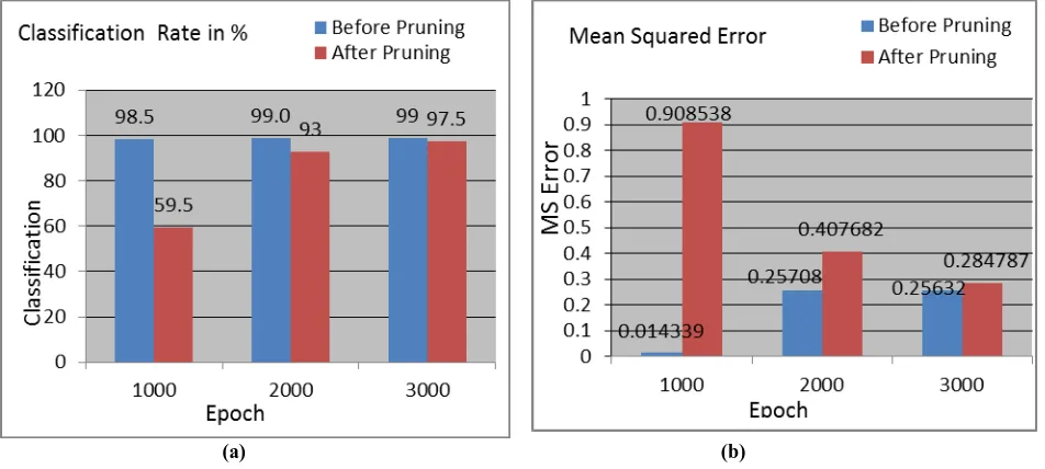
The network 14-30-10 is trained for 4000 epochs with learning rate of 0.25 and after each 1000 epochs the OBD pruning is carried out on the network. The parameters with saliency measures less than a chosen thresholdare removed. Empirically a threshold is selected as 0.0001. After 1000 epoch a classification rate of 98.5% and MSE of 0.014339 is observed in the network. At this point, the OBD is applied and 48 parameters with the saliency less than the threshold are removed from the network. Due to pruning the network’s performance is dropped and a classification rate of 59.5% and MSE of 0.908538 is observed. However the network is continued to train without 48 parameters in it, the network shows good learning behavior and at 2000 epoch a classification rate of 99.0% and MSE of 0.25708 is obtained.
Table. 1. Parameters removed. OBD
Applied Epoch
Number of Parameters Removed
1 1000 48
2 2000 15
3 3000 11
At 2000th epoch, OBD pruning method is applied second time and 15 parameters are removed. A classification rate of 93.0% and MSE of 0.407682 is observed as a result of removal of these parameters. Further network is subjected to training. At 3000th epoch OBD is applied and 11 parameters are removed. Due to this classification rate of 97.5% and MSE of 0.284787 is observed. The number of parameters are removed after each 1000 epoch has been shown in Table 1.
[image:5.595.335.523.487.563.2]effect on the network’s performance. At the end of 4000 epochs a classification rate of 98.3% and MSE of 0.164332 is observed in the network.
6.2 Feed-Forward Network Integrated With
BUF
A network architecture having 14 input neurons, 10 output neurons and 3 hidden layer having 15 neurons, is trained for 2000 epochs with learning rate 0.25. The network consists of 865 parameters (810 weights and 55 bias) to fit the input-output mapping. After each 5 epochs BUF algorithm is
employed on the network and behavior of integrated network is analyzed.
The Fig. 6(a) shows the number of nodes frozen and Fig. 6(b) shows number of nodes pruned when the algorithm is applied on the network. Freezing of a node depends upon its last 5 error signals. If the error signal did not reduced in last 5 observations then the node is frozen. The Table 2 shows few nodes which are frozen during learning phase. For last 5 epochs error rate for the node 3 in the layer 4 did not reduce and therefore it is frozen at epoch 50 for duration of 1 epoch. Other few node which are frozen are shown in Table 2.
(a) (b)
Fig. 5: (a) Classification rate. (b) MSE during nodes pruning by OBD.
(a) (b)
Fig. 6: (a) Number of nodes frozen.(b) Number of nodes pruned due to application of BUF.
Frozen Nodes/Epoch
0 0.2 0.4 0.6 0.8 1 1.2
5
155 305 455 605 755 905
1055 1205 1355 1505 1655 1805 1955
Epoch
N
o
.
o
f
fr
o
ze
n
n
o
d
e
s
Removed Nodes/Epoch
0 0.5 1 1.5 2 2.5 3 3.5
5
165 325 485 645 805 965
1125 1285 1445 1605 1765 1925 Epoch
N
o
.
o
f
re
m
o
v
e
d
n
o
d
e
[image:6.595.54.530.210.424.2] [image:6.595.67.531.520.711.2]Table 2: Duration and Error Signals of a frozen node.
Epoch Layer NodeNo Duration Error Rate Of Last 5 Epochs
50 4 3 1 154.147516 1.06687 0.659187 63.219315 15.053593
135 3 10 1 6.983052 11.31784 7.557551 29.177522 2.318116
145 4 9 1 8.63546 25.797278 33.757988 65.79339 45.151762
255 3 7 1 138.316476 7.263404 24.938371 2.470866 14.578681
275 2 11 1 32.531938 46.325595 0.263319 11.066844 11.058986
595 4 11 1 50.885971 226.640126 23.34371 14.063278 16.564948
625 4 10 1 77.438726 26.088658 83.256769 34.750765 103.217916
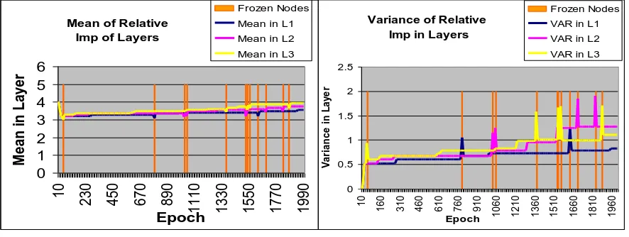
To decide the pruning in a layer, the mean and variance of relative importance of each node are observed. The Fig. 7(a) shows the mean and Fig 7(b) shows the variance of the relative importance of all the nodes in hidden layers. In BUF algorithm, the basic idea underlying the node removal is to analyze the freezing behavior of a hidden node and remove the node if it freezes very frequently. If a node is frozen in a layer then mean of relative importance in that layer decreases and variance of relative importance increases, which is readily be observed in Fig. 7.
The Table 3 specifies the nodes that are pruned from network during different epochs. Total number of nodes pruned is 9. During epoch 15, 15th node in layer 2 is pruned, as its relative importance was 4. During epoch 15, 20, 25 remaining 8 nodes were pruned as shown in the Table 3.When the nodes are frozen during the training, it affects the performance of the network. The Fig. 8(a) shows effect of freezing of nodes on the classification rate. The effect of freezing of nodes on MSE is depicted in the Fig. 8(b). Whenever nodes are frozen a slight decrease in classification rate and increase in MSE is observed.
[image:7.595.72.515.340.507.2](a) (b) Fig. 7(a) The mean. (b) The variance of all the nodes in layers.
Table 3: Nodes pruned during epochs
Epoch 15 15 15 20 20 20 25 25 25
Layer 2 3 4 2 3 4 2 3 4
Node 15 15 15 14 14 14 13 13 13
R 4 4 4 4 4 4 4 4 4
Variance of Relative Imp in Layers
0 0.5 1 1.5 2 2.5
10 160 310 460 610 760 910
1060 1210 1360 1510 1660 1810 1960 Epoch
V
a
ri
a
n
c
e
i
n
L
a
ye
r
Frozen Nodes
VAR in L1
VAR in L2
VAR in L3
Mean of Relative Imp of Layers
0 1 2 3 4 5 6
10
230
450
670
890
1110
1330
1550
1770
1990
Epoch
M
e
a
n
i
n
L
a
y
e
r
Frozen Nodes
Mean in L1
Mean in L2
(a)
(b)
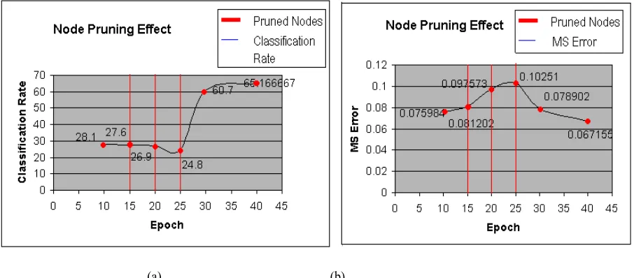
Fig.8: (a) Classification rate. (b) MSE in network observed after applying the BUF.The performance of the network when node pruning is analyzed. The Fig. 9(a) shows classification rate and Fig. 9(b) shows MSE when pruning is performed. On removing nodes from the network the classification rate decreases and MSE increase. At epoch 10 the classification rate of 28.1% and MSE of 0.07598 are observed. When three nodes are pruned at epoch 15 the classification rate decreases to 27.6% and MSE increased to 0.081202. Similarly observation can be made in Fig. 9 at epochs 20 and 25 as 6 more nodes are pruned. But a rapid increase in classification rate and decrease in MSE of 60.7% and 0.078902 respectively are observed immediately after node pruning. This indicates the BUF algorithm remove least important nodes from the network.
Determining the appropriate size of a neural network to solve a given problem is one of the important issues while designing the neural network. Dynamic learning algorithms have been proposed by researcher to overcome trail-and-error scheme of selecting the topology. Aim of the dynamic learning algorithms are to find the adequate size of neural networks during learning phase. The dynamic learning based on pruning involves in eliminating few elements to determine appropriate size of the neural network. In this paper the OBD and BUF algorithms are integrated separately with multilayer feed-forward neural network and their learning behavior has been analyzed.
(a) (b)
Fig. 9(a) Classification rate.(b) MSE in network observed between epochs 10 to 40.
7. CONCLUSION
The OBD method involves in removing least saliency parameters from the neural network. The BUF algorithm identifies nodes whose contribution to convergence fall below a certain threshold and freezes them. When a node is frozen very oftenly and number of times a node is frozen exceeds a certain limit then it is permanently removed from the network. The experiments have been conducted on feed-forward neural network to recognize MNIST handwritten numerals. It has
been observed that wheneverredundant elements are removed from the network during training its performance reduces which is indicated in decrease in classification rate and increases in MSE. However as the training continues the neural network shows the ability to learn with fewer elements in it. From experiments it is also observed that as the network reaches its local minima, applying OBD or BUF and pruning few elements has less effect on its performance than the initial phase of learning. Thus on integrating pruning methods such as OBD or BUF with multilayer feed-forward network allows
Classification Rate per Epoch
0 20 40 60 80 100 120
10 160 310 460 610 760 910
1060 1210 1360 1510 1660 1810 1960
Epoch
C
la
ss
if
ic
a
ti
o
n
R
a
te
Frozen Nodes Classification Rate
MS Error
per Epoch
0
0.02
0.04
0.06
0.08
0.1
0.12
0.14
10
240
470
700
930
1160
1390
1620
1850
Epoch
M
S
Er
ro
r
Frozen Nodes
[image:8.595.65.536.78.274.2] [image:8.595.70.523.429.628.2]to determine optimum sized network by reducing number of elements from it during the learning phase.
8. REFERENCES
[1] Giovanna Castellano, 1997.Ann Maria Fanelli and MarcellocPelillo, An Iterative Pruning Algorithm for Feed forward Neural Networks, in IEEE Trans. on Neural Network, 8, (3),519-531.
[2] Russel Reed, 1993.Pruning Algorithms- A Survey, in IEEE Trans. on Neural Network, 4, (5), 740-747. [3] Timothy Masters, 1993. Practical Neural Network
Recipes in C++ Academic Press, Inc, Harcourt Brace & Company Publisher, Boston San Diego New York. [4] E.B. Baum and D.Haussler, 1989.What size net gives
valid generalization? inNeural Computation, 1, 151-160. [5] J.Denker, D.Schwartz, B.Wittner, S.Solla, R.Howard,
L.Jackel and J.Hopfield, 1987.Large automatic learning, rule extraction, and generalization, in Complex Systems, 1, 877-922.
[6] Y.LeCun, 1989.Generalization and network design strategies, in Connectionism in Perspective, R.Pfeifer, Z.Schreter, F.Fogelman-Soulie and L.Steels, Eds, Amsterdam: Elsevier, 143-155.
[7] Y. Le Cun, J.S. Denker, and S.A. Solla, 1990.Optima Brain Damage, in Advances in Neural Information Processing (2), D.S. Touretzky, Ed (Denver 1989), 598-605.
[8] B. Hassibi and D.G. Stork, 1993.Second-order derivatives for network pruning: Optimal Brain Surgeon, in Advances in Neural Information Processing Systems, S.J.Hanson, J.d.Cowan and C.L.Gileses San Mateo, CA: Morgan Kaufmann, 164-171.
[9] Sietsma, J., and R.J.F. Dow, 1991. Creating artificial neural networks that generalize, in Neural Networks, vol. 4,(1), 67-79.
[10]Mozer, M.C., and P. Smolensky,1989.Skeletonization: A technique for trimming the fat from a network via relevance assessment, in D.S. Touretzky, editor, Advances in Neural Information Processing Systems (Denver, 1988) (1), Morgan Kaufmann, San Mateo, 107-115.
[11]Ali Farzan and Ali A. Ghorbani, 2001.The Bottom-Up Freezing: An Approach to Neural Engineering, in Proceedings of Advances in Artificial Intelligence: 14th Biennial Conference of the Canadian Society for Computational Studies of Intelligence, AI, Ottawa, Canada, 317 – 324.
[12]Giorgio Corani, Giorgio Guariso, 2005. An application of pruning in the designof neural networks for real time flood forecasting, in Journal Neural Computing and Applications, 14, (1), 66-77.
[13]P. Galerne , K. Yao , G. Burel1998.New Neural Network Pruning and its application to sonar Imagery, in Conference IEEE-CESA’98, Hammamet, Tunisia, April 1-4.
[14]Kenji Suzuki, Isao Horiba, Noboru Sugie, 2001. A Simple Neural Network Pruning Algorithm with Application to Filter Synthesis, in Neural Processing Letters, 13, (1), 43-53.