BIROn - Birkbeck Institutional Research Online
Lozin, V. and Razgon, Igor and Zamaraev, V. (2017) Well-quasi-ordering
versus clique-width. Journal of Combinatorial Theory Series B 130 , pp.
1-18. ISSN 0095-8956.
Downloaded from:
Usage Guidelines:
Please refer to usage guidelines at or alternatively
Well-quasi-ordering versus clique-width
∗Vadim Lozin† Igor Razgon‡ Viktor Zamaraev§
Abstract
Does well-quasi-ordering by induced subgraphs imply bounded clique-width for hereditary classes? This question was asked by Daligault, Rao, and Thomass´e [Well-quasi-order of relabel functions. Order, 27(3) (2010), 301–315]. We answer this question negatively by presenting a hereditary class of graphs of unbounded clique-width which is well-quasi-ordered by the induced subgraph relation. We also show that graphs in our class have at most logarithmic clique-width and that the number of minimal forbidden induced subgraphs for our class is infinite. These results lead to a conjecture relaxing the above question and to a number of related open questions connecting well-quasi-ordering and clique-width.
1
Introduction
In this paper, we study two seemingly unrelated notions: well-quasi-ordering and clique-width.
Well-quasi-ordering (wqo) is a highly desirable property and a frequently discovered concept
in mathematics and theoretical computer science [9, 14]. One of the most remarkable recent results in this area is the proof of Wagner’s conjecture stating that the set of all finite graphs is well-quasi-ordered by the minor relation [18]. This, however, is not the case for the induced subgraph relation, since it contains infinite antichains, for instance, the antichain of cycles. On the other hand, the induced subgraph relation may become a well-quasi-order when restricted to graphs in particular classes. Throughout this paper, we use the notion of well-quasi-ordering with respect to the induced subgraph relation only.
Clique-width is a much younger notion thanwqo. It was introduced in 1993 in [4] and it
generalizes another graph parameter, tree-width, which was studied in the literature for decades. Both parameters are important in algorithmic graph theory, as graphs of “low” tree- or clique-width admit efficient solutions for many problems which are generally intractable [5]. Typically, “low” means “bounded by a constant”. However, a logarithmic upper bound on clique-width does the same job, i.e., it provides polynomial-time algorithms. The notion of clique-width was also generalized from graphs to logical structures of arbitrary signature and cardinality [3].
Very little suggests that there is anything in common between these two notions, well-quasi-ordering and clique-width. One hint comes from the fact that the first non-trivial step towards the proof of Wagner’s conjecture was made for graphs of bounded tree-width [17]. In the case
∗
The results of Sections 3.1 and 4.1 are to appear in a conference version [11] of the paper.
†
Mathematics Institute, University of Warwick, Coventry CV4 7AL, UK. E-mail: [email protected].
‡
Department of Computer Science and Information Systems, Birkbeck, University of London, E-mail: [email protected]
§
of induced subgraphs, the first non-trivial result was obtained by Damaschke who showed in [8] that cographs are well-quasi-ordered by induced subgraphs. What is interesting is that cographs are precisely the graphs of clique-width at most 2 (see e.g. [6]). In [16], Petkovˇsek introduced an infinite family ofwqograph classes under the namek-letter graphs, and again all of them turned
out to be of bounded clique-width. Recently, many new wqo classes have been discovered in
the literature (see e.g. [1, 12, 13]), and the same phenomenon was observed in all of them. This discussion naturally leads to the following question:
Question 1. Does well-quasi-ordering imply bounded clique-width?
This question was formally stated by Daligault, Rao, and Thomass´e in [7]. More precisely, they stated it for hereditary classes, i.e., classes closed under taking induced subgraphs. The restriction to hereditary classes is natural for graphs of bounded width, since the clique-width of a graph is never smaller than the clique-clique-width of any of its induced subgraphs [6]. An important feature of hereditary classes is that each of them can be characterized by a unique set of minimal forbidden induced subgraphs. If this set is finite, we call the class finitely defined.
In the present paper, we answer Question 1 negatively by exhibiting a hereditary class of graphs of unbounded clique-width, which is well-quasi-ordered by the induced subgraph relation. We call graphs in our class the power graphs.
Our negative result is not the end of the story about well-quasi-ordering and clique-width, as the relationship between these two notions is not exhausted by Question 1. In the same paper [7], Daligault, Rao, and Thomass´e propose the following conjecture.
Conjecture 1. Every 2-well-quasi-ordered hereditary class of graphs has bounded clique-width.
The notion of 2-well-quasi-ordering deals with a restriction of the induced subgraph relation to graphs whose vertices are colored with two colors, in which case the relation is required to respect the colors. Clearly, 2-well-quasi-ordering implies well-quasi-ordering and therefore Conjecture 1 is a restriction of Question 1.
The example of power graphs does not destroy Conjecture 1, as graphs in this class are not 2-well-quasi-ordered. We derive this conclusion in a non-constructive way by showing that the class of power graphs isnotfinitely defined and combining this result with the following lemma proved by Daligault, Rao, and Thomass´e in [7].
Lemma 1. Any 2-well-quasi-ordered hereditary class is finitely defined.
The above discussion suggests another restriction of Question 1: does well-quasi-ordering imply bounded clique-width for finitely defined hereditary classes? According to Lemma 1, this restriction generalizes Conjecture 1. We believe that this generalization is true and formally state it as a conjecture in the concluding section of the paper. In the same section, we discuss several related open questions connecting well-quasi-ordering with clique-width. In particular, we ask about the speed of growth of clique-width in well-quasi-ordered classes of graphs. For power graphs, we show that the speed is bounded by a logarithmic function, which keeps our class in the area of tractability for many algorithmic problems, in spite of the negative answer to Question 1.
function of the number of vertices (Section 3.2). Section 4 is devoted to the notion of wqoand
proves two results: the class D is well-quasi-ordered (Section 4.1) but not 2-well-quasi-ordered (Section 4.2). Section 5 concludes the paper with a discussion and a number of open problems.
2
The power graphs
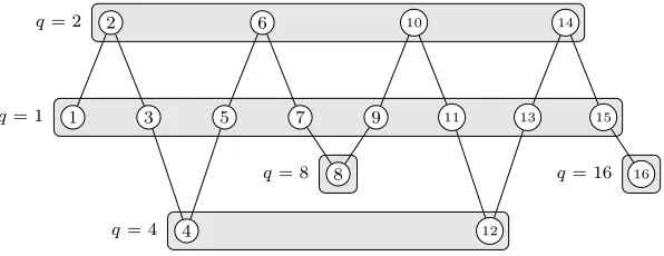
Let P be a path with vertex set{1, . . . , n}with two vertices iand j being adjacent if and only if|i−j|= 1. For a vertexi, the largest number of the form 2k that dividesiis called thepower of iand is denoted by q(i). For example,q(5) = 1, q(6) = 2, q(8) = 8, q(12) = 4.
To define the class of power graphs, we add toP edges connecting iand j whenever q(i) = q(j) and denote the resulting graph byDn. Figure 1 illustrates the graph D16.
q= 1
q= 2
q= 8 q= 16
q= 4 1
2
3
4 5
6
7
8 9
10
11
12 13
14
15
[image:4.612.167.465.244.359.2]16
Figure 1: The graphD16. To avoid shading the picture with many edges, the power cliques are represented as gray rectangular boxes.
By definition, the edgesE(Dn)\E(P) form a set of disjoint cliques each consisting of vertices
of the same power. We call these cliquespower cliques, and say that a power cliqueQcorresponds to 2k if it consists of vertices of power 2k. We callP thebody ofDn, the edges ofE(P) thepath
edges, and the edges ofE(Dn)\E(P) theclique edges.
Definition 1. We define D to be the class of all graphs Dn, n ∈ N, and all their induced
subgraphs and call graphs in D the power graphs.
Given a graphGisomorphic to a graph inD, among all possible sets of integers yielding an induced subgraph of some graphDnisomorphic toG, we pick one arbitrarily and identifyV(G)
with this set.
Any set of consecutive integers will be called an interval and any subgraph of Dn induced
by an interval will be called a factor. The number of elements in an interval inducing a factor is thelengthof the factor. The vertex set of every graphG∈ D can be split into maximal intervals and we call the subgraphs of Ginduced by these intervalsfactor-componentsofG. We say that a vertexu of a factorF ismaximal ifq(u)≥q(v) for each vertex v ofF different fromu.
The following statements show that every factorF has exactly one maximal vertex, moreover the power of any other vertexv ofF is bounded by the length ofF, and is uniquely determined by the difference between v and the maximal vertex.
Lemma 2. Every factor F contains exactly one maximal vertex.
the vertex 2k(p+ 1). Clearly p+ 1 is an even number and hence q(2k(p+ 1)) ≥ 2k+1, which contradicts the maximality of 2k.
Lemma 3. LetF be a factor of length at mostc. Ifvis a vertex ofF different from its maximal vertex m, then q(v) =q(|m−v|). In particular, q(v)< c.
Proof. Assume that v > m. Let k1, p1, k2, p2 be such that m = 2k1p1 and v−m = 2k2p2, with p1, p2 being odd numbers. Observe that k2 < k1, since otherwise v = 2k1p1 + 2k2p2 = 2k1(p1+ 2k2−k1p2), where p1 + 2k2−k1p2 is a natural number. Therefore, q(v) ≥ 2k1 = q(m), which contradicts either the maximality of m or Lemma 2. Consequently, v = 2k1p
1+ 2k2p2 = 2k2(2k1−k2p
1+p2), where 2k1−k2p1+p2is an odd number. Hence,q(v) = 2k2 =q(v−m). Finally, since the length ofF is at mostc, we conclude thatv−m < c, and thereforeq(v) =q(v−m)< c.
The case whenv < mis proved similarly.
Corollary 1. Let F be a factor of length at most c. If m is a vertex of F with q(m)≥c, then m is the maximal vertex of F.
3
Clique-width of power graphs
The clique-width of a graph G, denoted cwd(G), is the minimum number of labels needed to construct the graph by means of the four graph operations:
• creation of a new vertex with a label,
• disjoint union of two labeled graphs,
• connecting vertices with specified labelsi andj,
• renaming label ito labelj.
Every graph G can be constructed by means of these four operations, and the process of the construction can be described either by an algebraic expression or by a rooted binary decom-position tree, whose leaves correspond to the vertices of G, the root corresponds to G, and the internal nodes correspond to the union operations. In Section 3.1, we show that the clique-width of graphs inDis unbounded, i.e., there is no constant bounding the clique-width of graphs inD. On the other hand, in Section 3.2 we show that the clique-width of graphs in D, as a function of the number of vertices, grows at most logarithmically.
3.1 Clique-width is unbounded in D
Given a graph G and a subset U ⊂ V(G), we denote by U the set V(G)−U. We say that two vertices x, y ∈ U are U-similar if N(x)∩U = N(y)∩U, i.e., if x and y have the same neighbourhood outside ofU. Clearly, theU-similarity is an equivalence relation and we denote the number of similarity classes ofU byµG(U). Also, we denote
µ(G) = min 1 3n≤|U|≤
2 3n
µG(U),
wheren=|V(G)|. Our proof of the main result of this section is based on the following lemma.
Proof. LetT be a decomposition tree constructing Gwithcwd(G) labels,ta node ofT, andUt
the set of vertices ofGthat are leaves of the subtree ofT rooted at t. It is known (see e.g. [15]) that cwd(G) ≥µG(Ut) for any node t of T. According to a well known folklore result, binary
tree T has a node t such that 13|V(G)| ≤ |Ut| ≤ 23|V(G)|, in which case µG(Ut) ≥µ(G). Hence
the lemma.
LetU ⊆V(Dn), and letP be the body ofDn. We denote byPU the subgraph ofP induced
by U. In other words, PU is obtained from Dn[U] by removing the clique edges. Since P is a
path, PU is a graph every connected component of which is a path.
In order to use Lemma 4 for proving the main result of the section we will show thatµDn(U)
is ‘large’ whenever bothU and U are ‘large’. Note that ifPU hascconnected components, then PU has at leastc−1 connected components. This allows us to distinguish between two cases: 1) bothPU and PU have many connected components; 2) bothPU andPU have a limited number of connected components. The former case is considered in the following lemma.
Lemma 5. If PU has c+ 1connected components, then µDn(U)≥c/2.
Proof. In thei-th connected component ofPU,i≤c, we choose the last vertex (listed along the path P) and denote it by ui. The next vertex of P, denoted ui, belongs to U. This creates a
matching of sizecwith edges (ui, ui). Note that none of (ui, uj) is a path edge fori < j. Among
the chosen vertices ofU at least half have the same parity. Their respective matched vertices of U have the opposite parity. Since the clique edges connect only the vertices of thesame parity, we conclude that at least c/2 vertices of U have pairwise different neighbourhoods in U, i.e., µDn(U)≥c/2.
Now we consider the case where both PU and PU have a limited number of connected components. Taking into account the definition ofµ(G) and Lemma 4 we can assume that both U and U are ‘large’, and hence each ofPU andPU has a ‘large’ connected component. In order to address this case we use the following lemma which states that a large number of power cliques intersecting both U and U implies a large value ofµDn(U).
Lemma 6. If there exist c different power cliques Q1, . . . , Qc each of which
(1) corresponds to a power of 2 greater than 1 and
(2) intersects both U andU,
then µDn(U)≥c.
Proof. Letui and ui be some vertices in Qi, which belong to U and U, respectively. Since all
the vertices inM ={u1, u1, . . . , uc, uc}are even and two even vertices are adjacent in Dn if and
only if they belong to the same power clique, M induces a matching in Dn with edges (ui, ui),
i = 1, . . . , c. This implies that u1, . . . , uc have pairwise different neighbourhoods in U, that is
µDn(U)≥c.
The only remaining ingredient to prove the main result of this section is the following lemma.
Proof. The statement easily follows from the fact that for any k ∈ {1, . . . , c}, vertices v with q(v) = 2k are of the formv= 2k(2p+ 1). In other words, they occur in P with period 2k+1.
Now we are ready to prove the main result of this section.
Theorem 1. Let n and c be natural numbers such that n ≥ 3((2c+ 1)(2c+1−1) + 1). Then cwd(Dn)≥cand hence the clique-width of graphs in D is unbounded.
Proof. LetU be an arbitrary subset of vertices of Dn, such that n3 ≤ |U| ≤ 23n. Note that the
choice ofU implies that the cardinalities of bothU andU are at least n3 ≥(2c+ 1)(2c+1−1) + 1. IfPU has at least 2c+1 connected components, then by Lemma 5µ
Dn(U)≥c. OtherwisePU
has less than 2c+ 1 connected components andPU has less than 2c+ 2 connected components. By the pigeonhole principle, each of the graphs has a connected component of size at least 2c+1. Clearly, these connected components are disjoint subpaths ofP. By Lemma 7, the power cliques corresponding to 21, . . . ,2c intersect both U and U, and hence, by Lemma 6,µDn(U)≥c.
SinceU has been chosen arbitrarily, we conclude thatµ(Dn)≥c, and therefore, by Lemma 4,
cwd(Dn)≥c, as required.
3.2 Power graphs have at most logarithmic clique-width1
In this section, we show that for any n-vertex graphG in D the clique-width ofG is bounded from above by 2dlogne+ 8. We start with two auxiliary lemmas.
Lemma 8. For any natural n, the clique-width of Dn is at mostdlog(n+ 1)e+ 2.
Proof. We obtain graphDn by constructing consecutively labeled graphs H1, ..., Hn, where Hi
is isomorphic to Di. During the construction process of Hi we only use labels from the set
{a |2a ≤i, a∈N0} and two more auxiliary labels x, y. Moreover, if i < n, then vertex iof Hi
is labeled byx, otherwise a vertexj of Hi is labeled bya, where q(j) = 2a.
Let H1 be the graph with V(H1) = {1}, and the unique vertex of H1 is labeled by x. For everyi= 2, . . . , n, we consecutively perform the following steps:
1. create vertex iwith label y;
2. defineHi to be a disjoint union ofHi−1 and vertex i;
3. in Hi add an edge between the only vertex with label x (i.e., vertex i−1) and the only
vertex with label y (i.e., vertex i);
4. inHi assign to vertexi−1 labela, whereq(i−1) = 2a;
5. inHi add the edges between the only vertex with labely(i.e., vertexi) and all the vertices
with label a, whereq(i) = 2a;
6. if i < n, then assign to vertex ilabelx, otherwise assign toilabel a, whereq(i) = 2a.
It is easy to verify that Hn is equal to Dn. Moreover, the only used labels in the above
procedure are x, y and integers from the set {a | 2a ≤ n, a ∈ N0}. Since the latter set has dlog(n+ 1)e elements, we obtain the desired result. Notice that in Hn two vertices have the
same power if and only if they have the same label.
Lemma 9. Let F be a factor of length n. Then the clique-width of F is at most dlogne+ 4.
Proof. Taking into account Lemma 8 and the fact that the clique-width of an induced subgraph of a graph does not exceed the clique-width of the graph, it is sufficient to show that F is an induced subgraph of D3n.
Let i, j and m be the first, the last, and the maximal vertices of F, respectively. Let also c1 =m−i,c2 =j−m,c= max{c1, c2}, and let 2r be the smallest power of 2 exceeding c. We
claim that functionf :V(F)→V(D2r+c
2), given by
f(m+v) = 2r+v forv∈ {−c1, . . . ,−1,0,1, . . . , c2}
is a subgraph isomorphism2 from F to D2r+c
2. Note that by Lemma 2 each of F and D2r+c2 has a unique maximal vertex. Further, by the definition, f maps consecutive vertices of F to consecutive vertices of D2r+c
2, and the maximal vertex of F to the maximal vertex of D2r+c2. Moreover, by Lemma 3 function f preserves powers of non-maximal vertices. Now, since in a power graph two vertices are adjacent if and only if either they are consecutive integers, or they have the same power, we conclude that f is a subgraph isomorphism fromF toD2r+c
2. Finally, since 2r≤2c, we have 2r+c2 ≤3c≤3n, and the result follows.
Theorem 2. Let G be an n-vertex graph from D. Then the clique-width of G is at most 2dlogne+ 8.
Proof. Denote bytthe length of a longest factor-component inG. We will show that Gcan be constructed by the clique-width operations using at most 2(dlogte+ 4) different labels. Since t ≤ n, this will give the result. By Lemma 3, powers of all vertices in G, except possibly the maximal vertices of some factor-components, are less than t. In particular, in the construction of a factor-component ofG, provided by Lemmas 8 and 9, all non-maximal vertices are labeled by non-negative integers less than dlogte, and without loss of generality we will assume that if the unique maximal vertex has power at least t then it is always labeled by dlogte. We will distinguish between two types of maximal vertices:
1. maximal vertices of power less than t. These vertices may have non-maximal neighbours outside their factor-components. We will treat them as any other non-maximal vertex, that is, for a vertex of power 2i we will use label i;
2. maximal vertices of power at least t. It follows from Corollary 1 that outside their factor-components these vertices are adjacent only to other maximal vertices of the same power. For all of them we will use one common label dlogte. To do this we will need to con-struct independently each of the subgraphs induced by vertices of factor-components with maximal vertices of the same power, and successively combine these subgraphs with each other.
For convenience, letk=dlogte+ 4.
Let us first assume that the maximal vertices of all factor-components inG have the same power. We will prove by induction on the number s of factor-components that G can be con-structed using 2k labels in such a way that at the end of the procedure the vertices of G are assigned labels from the set {0, . . . ,dlogte} with a vertex of power 2i being assigned label i if
2i < t, and label dlogteotherwise. If Ghas only one factor, then it can be constructed using at mostklabels by Lemma 9. Moreover, it follows from the proof of Lemma 8 that the construction possesses the desirable properties. Let nows >1. Assume that we can properly construct every graph with less than s factor-components, and let G has s factor-components. Denote by F a factor-component of G, and let G0 be the subgraph of G induced by the vertices outside of F. Using the induction hypothesis and an appropriate relabeling of the vertices of graphF, we can assume that bothG0 andF have been constructed independently using at most 2kdifferent labels in such a way that the vertices of G0 are assigned labels from the set{0, . . . ,dlogte}, ver-tices ofF are assigned labels from the set {k, . . . , k+dlogte}, and for everyi∈ {0, . . . ,dlogte} the vertices ofG0 with labelihave the same power as the vertices ofF with labelk+i. Now, to constructGwe take the disjoint union ofG0 andF, and for everyi∈ {0, . . . ,dlogte}successively do the following operations:
1. add all edges between the vertices with label iand the vertices with labelk+i;
2. rename label k+ito label i.
The general case is proved similarly, except that the induction goes over the number p of different powers of maximal vertices in factor-components of G. Specifically, we will show by induction onpthat the clique-width ofGis at most 2k, andGcan be constructed using at most 2k labels in such a way that at the end of the procedure a vertex of power 2i is assigned label i if 2i < t, and every (maximal) vertex of power at least t is assigned label dlogte. The above discussion provides the base case, whenp= 1. Let nowp >1. Suppose that all graphs in which powers of maximal vertices take less than p different values admit the desirable construction, and consider a graph Gwhose powers of maximal vertices of factor-components take exactly p different valuesq1, . . . , qp. LetG1 be the subgraph ofGinduced by the vertices of those
factor-components whose maximal vertices have one of the powers q1, . . . , qp−1. Similarly, let G2 be the subgraph of G induced by the vertices of those factor-components whose maximal vertices have power qp. Using the induction hypothesis and an appropriate relabeling of the vertices of
graph G2, we can assume that both G1 and G2 have been constructed independently using at most 2k different labels in such a way that the vertices of G1 are assigned labels from the set {0, . . . ,dlogte} with dlogtebeing the label of the maximal vertices of power at least t, and the vertices ofG2 are assigned labels from the set{k, . . . , k+dlogte}withk+dlogtebeing the label of the maximal vertices of power at leastt, and for every i∈ {0, . . . ,dlogte −1} the vertices of G1 with labeliand the vertices ofG2with labelk+ihave the same power 2i. Now, to construct Gin a suitable way we first take the disjoint union of the constructed graphs G1 and G2. Then rename labelk+dlogteto labeldlogte, and for every i∈ {0, . . . ,dlogte −1}successively do the following operations:
1. add all edges between the vertices with label iand the vertices with labelk+i;
2. rename label k+ito label i.
4
Power graphs and well-quasi-ordering
y≤x. Otherwise, x and y are incomparable. A set of pairwise comparable elements is called a chain and a set of pairwise incomparable elements anantichain. A quasi-order (W,≤) is a well-quasi-order if it contains neither infinite strictly decreasing chains nor infinite antichains. Since we deal with the induced subgraph relation on finite graphs, infinite strictly decreasing chains are impossible. Therefore, a class of graphs is well-quasi-ordered by the induced subgraph relation if and only if it contains no infinite antichains with respect to this relation. In Section 4.1, we show that graphs in D are well-quasi-ordered.
In Section 4.2, we deal with a more restrictive version of well-quasi-ordering known as k-well-quasi-ordering. A class of graphs X is said to be k-well-quasi-ordered if the set consisting of all vertex k-colored3 graphs from X is well-quasi-ordered by the induced subgraph relation respecting the colors. In other words, when we embed a graphH into a graphG as an induced subgraph we must map the vertices of H to vertices of Gof thesame color. In Section 4.2, we show that the class Dis not 2-well-quasi-ordered.
4.1 D is well-quasi-ordered
In the proof of the main result of this section, we apply a celebrated lemma due to Higman [10], which can be stated as follows. For an arbitrary setM, letM∗ be the set of all finite sequences of elements ofM. Any quasi-order≤onM defines a quasi-orderonM∗as follows: (a1, . . . , am)
(b1, . . . , bn) if and only if there exists a strictly increasing mapping f :{1, . . . , m} → {1, . . . , n}
such that ai ≤bf(i) for each i= 1, . . . , m.
Lemma 10. [10] If (M,≤) is a wqo, then (M∗,) is a wqo.
Since the induced subgraph relation contains no infinite strictly decreasing chains, to prove the main result we need to show that for each infinite sequence G =G1, G2. . . of graphs inD there arei, j such thatGi is an induced subgraph of Gj. First we prove the following auxiliary
lemma.
Lemma 11. Let G be a graph in D. Then there exists an integer t= t(G) such that for any n≥t every factor of Dn of length at least tcontains G as an induced subgraph.
Proof. Lets be the smallest number such thatG is an induced subgraph of Ds. We will show
that t = 5s satisfies the lemma. To this end it is enough to prove that any factor F of Dn
of length at least t contains Ds as an induced subgraph. By the transitivity of the induced
subgraph relation, this will imply that Gis an induced subgraph of F.
Let 2k be the smallest power of 2 larger than s. Clearly, 2k+1 ≤ 4s. Hence, by Lemma 7, among the first 4s vertices of F there is a vertex y with q(y) = 2k. Let F0 be the factor induced by the vertices of F starting at y+ 1. Since F is of length at least 5sand y is among the first 4svertices ofF, the length ofF0 is at leasts. Thus we can define an injective function f : V(Ds) → V(F0) as follows: f(z) = y+z for 1 ≤ z ≤ s. We claim that f is a subgraph
isomorphism from Ds to a subgraph of F. Clearly, f(z+ 1) =f(z) + 1 for 1≤z < s, hence it
remains to verify that adjacencies and non-adjacencies are preserved for verticesz1, z2ofDssuch
thatz2> z1+1. Clearly, in this casez1andz2are adjacent if and only ifq(z1) =q(z2). Moreover, sincef(z2)> f(z1)+1,f(z2) andf(z1) are adjacent if and only ifq(f(z1)) =q(f(z2)). Below we show thatq(f(z)) =q(z) for 1≤z≤sand henceq(z1) =q(z2) if and only ifq(f(z1)) =q(f(z2)), implying the lemma.
Indeed, f(z) = y+z = 2kp+ 2k1p1, where 2k1 = q(z) and p, p1 are odd numbers. Since 2k1 ≤s <2k,k
1 < k and hencey+z= 2k1(2k−k1p+p1), where 2k−k1p+p1 is an odd number. Consequently, q(y+z) = 2k1 =q(z), as required.
Lemma 12. If G contains graphs with arbitrarily long factor-components, then G is not an antichain.
Proof. Pick an arbitraryGiinG. By assumption,Gcontains a graphGj with a factor-component
F of length at least t(Gi), where t(Gi) is given by Lemma 11. By the same lemma, the graph
Gi is an induced subgraph ofF, and therefore is an induced subgraph of Gj.
From now on, we assume that the length of factor-components of graphs inG is bounded by some constantc=c(G). In what follows we prove that in this caseG is not an antichain as well.
LetF be a factor. In light of Lemma 2, we denote the unique maximal vertex ofF bym(F). Also, let s(F) be the smallest vertex of F. Now we define two equivalence relations on the set of factor graphs as follows. We say that two factors F1 and F2 are
• t-equivalent if they are of the same length and m(F1)−s(F1) =m(F2)−s(F2),
• `-equivalent ifq(m(F1)) =q(m(F2)).
For a non-negative integer iwe denote byLi the`-equivalence class such thatq(m(F)) = 2i for
every factorF in this class. We also order thet-equivalence classes (arbitrarily) and denote by Tj thej-th class in this order.
Lemma 13. Let F1, F2 be two t-equivalent factors. Then there exists an isomorphism f from F1 toF2 such that:
(a) f(m(F1)) =m(F2);
(b) q(f(v)) =q(v) for allv∈V(F1) except possibly for m(F1).
Proof. We claim that the function f that maps the i-th vertex of the factor F1 (starting from the smallest) to the i-th vertex of the factor F2 is the desired isomorphism. Indeed, property (a) follows from the condition that the factors aret-equivalent. Now property (a) together with Lemma 3 imply property (b). Finally, since adjacency between vertices in a factor is completely determined by their adjacency in the body and by their powers, we conclude that f is, in fact, an isomorphism.
For a graph G ∈ D, we denote by Gi,j the set of factor-components of G in Li∩Tj, and
define a binary relation ≤on graphs ofD as follows: G≤H if and only if |Gi,j| ≤ |Hi,j|for all
iand j (clearly in this definition one can be restricted to non-empty sets Gi,j).
Finally, for a constantc=c(G) we slightly modify the definition of≤ to≤c as follows. We say that a mapping h:N0 →N0 is c-preserving if it is injective and h(i) =ifor alli≤ blogcc. Then G≤cH if and only if there is a c-preserving mapping h such that|Gi,j| ≤ |Hh(i),j|for all
iand j. The importance of the binary relation ≤c is due to the following lemma.
Lemma 14. Suppose the length of factor-components of G andH is bounded by cand G≤cH.
Proof. We say that a factorF islow-poweredifF ∈Li, for somei≤ blogcc, i.e., ifq(m(F))≤c.
Also for a graphG we denote byF(G) the set of all its factor-components.
It can be easily checked that the definition of≤cimplies the existence of an injective function
φ:F(G)→ F(H) that possesses the following properties:
(1) φmaps each of the factors in F(G) to at-equivalent factor inF(H);
(2) F ∈ F(G) is a low-powered factor if and only ifφ(F) is;
(3) φpreserves power of the maximal vertex for each of the low-powered factors, i.e.,q(m(F)) = q(m(φ(F))) for every low-powered factorF ∈ F(G);
(4) for any two factors F1, F2 ∈ F(G), q(m(F1)) = q(m(F2)) if and only if q(m(φ(F1))) = q(m(φ(F2))).
To show that G is an induced subgraph of H we define a witnessing function that maps vertices of a factorF ∈ F(G) to vertices ofφ(F)∈ F(H) according to an isomorphism described in Lemma 13. This mapping guarantees that a factor F of G is isomorphic to the factorφ(F) ofH. Therefore it remains to check that adjacency relation between vertices in different factors is preserved under the defined mapping.
Note that adjacency between two vertices in different factors is determined entirely by the powers of these vertices. Moreover, Lemma 13 and property (3) of φ imply that our mapping preserves powers of all vertices except possibly maximal vertices of power more thatc. Therefore in order to complete the proof we need only to make sure that in graph Ga maximal vertex m of a factor F with q(m)> c is adjacent to a vertex v in a factor different fromF if and only if the corresponding images of m and v are adjacent inH.
Taking into account Corollary 1 we derive that a maximal vertexmwithq(m)> cis adjacent to a vertex v in a different factor if and only if v is maximal in that factor and q(m) = q(v). Now the desired conclusion follows from Lemma 13 and properties (2) and (4) of functionφ.
Lemma 15. The set of graphs in D in which factor-components have length at most c is well-quasi-ordered by the relation ≤c.
Proof. We associate with each graph G∈ D containing no factor-component of length greater thanc a matrix MG=m(i, j) with m(i, j) =|Gi,j|, where i∈N0, and j∈N.
Each row of this matrix corresponds to an `-equivalence class and we delete any row corre-sponding to Li withi > blogcc which is empty (contains only 0s). This leaves a finite amount
of rows (sinceG is finite).
Each column of MG corresponds to a t-equivalence class and we delete all columns
corre-sponding tot-equivalence classes containing factors of length greater thanc(none of these classes has a factor-component ofG). This leaves precisely c+12 columns inMG.
We define the relation on the set M of matrices constructed in this way as follows. For M1, M2 ∈ Mwe say thatM1M2if and only if there exists a strictly increasing mappingβfrom the index set of the rows ofM1to the index set of the rows ofM2 such thatm1(i, j)≤m2(β(i), j) for all i andj. In addition, ifβ is c-preserving, then we say thatM1 cM2. Note that if both
M1 and M2 have exactlyblogcc rows, then M1M2 is equivalent toM1 cM2.
by repeated applications of Higman’s lemma. First, we split each matrixM ∈ M into two sub-matrices M0 and M00 so that M0 contains the firstblogccrows and M00 contains the remaining rows. Let M0 ={M0|M ∈ M} and M00 ={M00|M ∈ M}.
To see that the set of matrices M0 is wqo by we apply Higman’s Lemma twice. First,
the set of rows iswqoby since all of them are finite words of equal length over the alphabet
of non-negative integers (which is wqo by the ordinary arithmetic ≤ relation). Second, the
set of matrices M0 is wqo by since each of them is a finite word over the alphabet of rows.
Similarly, the set of matrices M00 is
wqo by . Note that in both applications of Lemma 10
to M0 and in the first application to M00, we considered sets of sequences of the same length. Hence, in this case, Higman’s Lemma in fact implies the existence of two sequences one of which is coordinate-wise smaller than the other, exactly what we need in these cases.
Finally, since each matrix inMcan be considered as a word of two letters over the alphabet M0∪ M00, which iswqoby , and the relationsand c are equivalent on the set of matrices
M0, we conclude that Mis
wqo by c.
Combining Lemmas 12, 14, and 15, we obtain the main result of this section.
Theorem 3. The class D is well-quasi-ordered by the induced subgraph relation.
4.2 D is not 2-well-quasi-ordered
In this section, we prove that D is not 2-well-quasi-ordered. We obtain this result by showing that the classDis not finitely defined. The desired conclusion thatDis not 2-well-quasi-ordered will then follow from Lemma 1.
To prove that the class D is not finitely defined, we show that there are infinitely many minimal graphs that are not in D. For every integer k ≥3, we define Bk as a graph obtained
from a subgraph ofD3·2k induced by{1,2, . . . ,2k,5·2k−1,5·2k−1+ 1, . . . ,3·2k}by adding one
new edge (1,3·2k), which we call the binding edge of Bk. Similarly to graphs Dn, an edge of
Bk connecting two consecutive vertices, i.e., an edge of the form (i, i+ 1), is called apath edge.
In what follows, we show that the graphs Bk, k ≥3, are minimal forbidden induced subgraphs
for the class D. We start with technical lemmas.
Lemma 16. Let iand j be two different integers of the same power2k. Then |i−j| ≥2k+1.
Proof. Asq(i) =q(j) = 2k and i6=j, we conclude thati=r12k and j =r22k, wherer1 and r2 are two different odd integers. Then |r12k−r22k|= 2k|r1−r2| ≥2k+1.
Lemma 17. Let iand j be two integers with q(i) = 2k and q(j) = 2s, where k > s. Then i+j and |i−j|both have power 2s.
Proof. Leti =r12k and j =r22s, where r1, r2 are odd integers. Then i+j = 2s(r12k−s+r2) and |i−j| = 2s|r12k−s−r2|, and the lemma follows from the fact that both r12k−s+r2 and |r12k−s−r2|are odd.
Now we will show that none of the graphsBk, k≥3, belongs to D.
Lemma 18. For everyk≥3, the graph Bk does not belong to D.
Proof. Suppose to the contrary that there is an integer n and a function f :V(Bk) → V(Dn)
such that f is a subgraph isomorphism from Bk toDn. Note that the vertices of any clique of
by f to a clique of Dn, the images of all odd vertices of Bk have the same power. Moreover,
since every even vertex inBkhas at most two odd neighbours, the power of its image is different
from that of images of odd vertices. This means that all the path edges and the binding edge of Bk are mapped to path edges inDn. Hence, the image of V(Bk) forms an interval, and we
denote byF the factor ofDn induced by this interval. Note thatBkhas a unique largest clique,
namely the clique formed by the odd vertices. Similarly, becauseF is a factor of length at least |V(Bk)| ≥ |V(B3)| = 13, it has a unique largest clique, namely the clique formed by its odd
vertices. Therefore, as the largest clique is an invariant, the odd vertices of Bk are mapped to
the odd vertices ofF, and, hence,f preserves parity of the vertices. Furthermore, since in both Bk and F even vertices are adjacent if and only if they have the same power, we conclude that
v, u∈V(Bk) have the same power if and only iff(v), f(u) have the same power.
Now, sinceBk hask+ 1 cliques corresponding to different powers with at least two vertices
in each clique, there are two different verticesv, u∈V(Bk) whose imagesf(v) andf(u) have the
same power 2r withr≥k. Finally, as the image ofV(Bk) forms an interval of length 3·2k−1+ 1,
we have |f(v)−f(u)| ≤3·2k−1 <2k+1, which contradicts Lemma 16.
In the following lemma, we show that all graphsBk, k≥3, are in fact minimal forbidden.
Lemma 19. For every k ≥ 3, the graph Bk is a minimal forbidden induced subgraph for the
class D.
Proof. Taking into account Lemma 18, it is sufficient to prove that for every vertex v∈V(Bk)
the graphGv =Bk\ {v}belongs toD. Clearly, this is true ifvis one of the ends of the binding
edge, i.e if v ∈ {1,3·2k}. For all other vertices v, we will provide a subgraph isomorphism f from Gv to some graph inD.
First, assume thatv∈ {2, . . . ,2k}. We define f :V(Gv)→V(D2k+2) as follows:
f(i) = 3·2k+i, fori∈ {1, . . . , v−1};
f(i) =i, for all other i∈V(Gv).
Since v−1 < 2k, it follows from Lemma 17 that f preserves powers. Also, it is easy to see thatf maps consecutive vertices ofGv to consecutive ones. Moreover, only two non-consecutive
vertices ofGv, namely 1 and 3·2k, become consecutive under f, which corresponds to mapping
of the binding edge (1,3·2k) to a path edge (3·2k,3·2k + 1). Therefore, f is a subgraph isomorphism from Gv toD2k+2.
Now let v ∈ {5·2k−1,5·2k−1+ 1, . . . ,3·2k−1}. We define f : V(Gv) → V(D13·2k−1) as follows:
f(i) = 3·2k−1+i, fori∈ {1, . . . ,2k};
f(i) =i−3·2k−1, fori∈ {v+ 1, . . . ,3·2k};
f(i) = 7·2k−1+i, fori∈ {5·2k−1, . . . , v−1}.
Note that the powers of the vertices of Gv are at most 2k. By Lemma 17, the function f
preserves powers that are at most 2k−2. There are at most two vertices of power 2k−1, namely 2k−1 and 5·2k−1, and they are mapped by f, respectively, to vertices 2k+1 and 3·2k+1 of power 2k+1. Also there are exactly two vertices of power 2k, namely 2k and 3·2k, and they are
consecutive vertices. Moreover, only two non-consecutive vertices of Gv, namely 1 and 3·2k,
become consecutive under f, which corresponds to mapping of the binding edge (1,3·2k) to a path edge (3·2k−1,3·2k−1+1). Therefore,f is a subgraph isomorphism fromG
vtoD13·2k−1. Combining Lemmas 18 and 19 with Lemma 1, we derive the following conclusion.
Theorem 4. The class D is not finitely defined and hence is not 2-well-quasi-ordered.
5
Concluding remarks and open problems
In this paper, we introduced a new hereditary class of graphs, the power graphs, and derived a number of properties of these graphs. In particular, we proved that
(1) the clique-width of power graphs is not bounded by any constant,
(2) the clique-width of power graphs is at most logarithmic in the number of vertices,
(3) the class of power graphs is well-quasi-ordered by the induced subgraph relation,
(4) the class of power graphs is not finitely defined and hence is not 2-well-quasi-ordered by induced subgraphs.
This sequence of results implies several conclusions. First of all, it provides a negative answer to Question 1 posed in [7]. Let us observe that this question is not trivial at all and the area where the answer to this question is positive includes a variety of graph classes. In particular, it includes all hereditary graph classes where the number of edges is bounded from above by a subquadratic function [2], or, equivalently, all hereditary graph classes forbidding some complete bipartite graph as a (not necessarily induced) subgraph. In view of these results, identifying the “area of positivity” of Question 1 becomes an important open problem. We believe that, in addition to the above classes, this area includes all finitely defined hereditary classes and propose this idea as a conjecture.
Conjecture 2. Well-quasi-ordering implies bounded clique-width for finitely defined hereditary classes of graphs.
According to Lemma 1, Conjecture 2 generalizes Conjecture 1. Whether this generalization is proper (i.e., strictly stronger) is another open question:
Question 2. Are there finitely defined hereditary classes which are well-quasi-ordered but not 2-well-quasi-ordered by induced subgraphs?
We conclude the paper with one more open question suggested by our results.
Question 3. What is the maximal speed of growth of clique-width in well-quasi-ordered classes of graphs?
A logarithmic bound on clique-width would have strong algorithmic consequences. In particular, many computational problems intractable for general graphs would be solvable in polynomial time for well-quasi-ordered classes. This is the case for power graphs, as we showed in Section 3.2. Finding a bound valid for all well-quasi-ordered classes remains a challenging open problem.
References
[1] A. Atminas, R. Brignall, N. Korpelainen, V. Lozin, and V. Vatter, Well-quasi-order for permutation graphs omitting a path and a clique.Electron. J. Combin., 22(2) (2015), Paper 2.20, 21 pp.
[2] A. Atminas, V. V. Lozin, and I. Razgon, Well-quasi-ordering, tree-width and subquadratic properties of graphs. CoRR, abs/1410.3260, 2014.
[3] A. Blumensath, A model-theoretic characterisation of clique width.Ann. Pure Appl. Logic, 142(1-3) (2006), 321–350.
[4] B. Courcelle, J. Engelfriet, and G. Rozenberg, Handle-rewriting hypergraph grammars. Journal of Computer and System Sciences, 46 (1993), 218–270.
[5] B. Courcelle, J. A. Makowsky, and U. Rotics, Linear time solvable optimization problems on graphs of bounded clique-width. Theory Comput. Syst., 33(2) (2000), 125–150.
[6] B. Courcelle and S. Olariu, Upper bounds to the clique width of graphs. Discrete Appl. Math, 101(1-3) (2000), 77–114.
[7] J. Daligault, M. Rao, and S. Thomass´e, Well-quasi-order of relabel functions. Order, 27(3) (2010), 301–315.
[8] P. Damaschke, Induced subgraphs and well-quasi-ordering. Journal of Graph Theory, 14(4) (1990), 427–435.
[9] A. Finkel and Ph. Schnoebelen, Well-structured transition systems everywhere! Theor. Comput. Sci., 256(1-2) (2001), 63–92.
[10] G. Higman, Ordering by divisibility in abstract algebras. Proceedings of the London Math-ematical Society, 2 (1952), 326–336.
[11] V. V. Lozin, I. Razgon, and V. Zamaraev, Well-quasi-ordering does not imply bounded clique-width. InProceedings of the 41st International Workshop on Graph-Theoretic Con-cepts in Computer Science, Lecture Notes in Computer Science, (2015), 351–359.
[12] N. Korpelainen and V. V. Lozin. Two forbidden induced subgraphs and well-quasi-ordering. Discrete Mathematics, 311(16) (2011), 1813–1822.
[13] N. Korpelainen, V. V. Lozin, Bipartite induced subgraphs and well-quasi-ordering.J. Graph Theory, 67(3) (2011), 235-249.
[14] J. B. Kruskal, The theory of well-quasi-ordering: A frequently discovered concept.J. Comb. Theory, Ser. A, 13(3) (1972), 297–305.
[15] V. V. Lozin and D. Rautenbach, The relative clique-width of a graph. J. Comb. Theory, Ser. B, 97(5) (2007), 846–858.
[17] N. Robertson and P. D Seymour, Graph minors. IV. Tree-width and well-quasi-ordering. J. Combin. Theory Ser. B, 48(2) (1990), 227–254.