A stochastic differential equation approach to the analysis of the UK 2016 EU referendum polls

BIROn - Birkbeck Institutional Research Online

Fenner, Trevor and Levene, Mark and Loizou, George (2018) A stochastic

differential equation approach to the analysis of the UK 2016 EU referendum

polls. Journal of Physics Communications , ISSN 2399-6528.

Downloaded from:

Usage Guidelines:

Please refer to usage guidelines at

or alternatively

Journal of Physics Communications

PAPER • OPEN ACCESS

A stochastic differential equation approach to the analysis of the UK

2016 EU referendum polls

To cite this article: Trevor Fenner et al 2018 J. Phys. Commun. 2 055022

View the article online for updates and enhancements.

J. Phys. Commun.2(2018)055022 https://doi.org/10.1088/2399-6528/aac347

PAPER

A stochastic differential equation approach to the analysis of the UK

2016 EU referendum polls

Trevor Fenner, Mark Levene1 _{and George Loizou}

Department of Computer Science and Information Systems Birkbeck, University of London London WC1E 7HX, United Kingdom

1 _{The author to whom any correspondence should be addressed}

E-mail:[email protected],[email protected]@dcs.bbk.ac.uk

Keywords:generative model, stochastic differential equations, time series, beta distribution, referendum polls

Abstract

Human dynamics and sociophysics suggest statistical models that may explain and provide us with

better insight into social phenomena. Here we propose a generative model based on a stochastic

differential equation that allows us to analyse the polls leading up to the UK 2016 EU referendum.

After a preliminary analysis of the time series of poll results, we provide empirical evidence that the

beta distribution, which is a natural choice when modelling proportions,

fi

ts the marginal distribution

of this time series. We also provide evidence of the predictive power of the proposed model.

1. Introduction

Recent interest in complex social systems, such as social networks, the world-wide-web, messaging networks and mobile phone networks(Barabási2016), has led researchers to investigate the processes that could explain the dynamics of human behaviour within these networks. Human dynamics is not limited to the study of behaviour in communication networks, and has a broader remit similar to the aims ofsociophysics(Galam2008, Sen and Chakrabarti2014) (also known associal physics), which uses concepts and methods from statistical physics to investigate social phenomena, opinion formation and political behaviour. A central idea here is that, in the context of statistical physics, individual humans can be thought of as‘social atoms’, each exhibiting simple individual behaviour and possessing very limited intelligence, but nevertheless collectively yielding complex social patterns(Bentley and Ormerod2011).

Social physics has a long history going back to the polymath Quetelet in the 19th century, who applied statistical laws to the study of human characteristics; for example, in deriving thebody mass index, he discovered that body weight is approximately proportional to the square of the body height(Eknoyan2008). The

foundations of 20th century social physics can be attributed to Stewart(Stewart1950), whose research was linked to applying gravitational potential theory to the geographic distribution of populations.

Polls impart important information to the public in the lead-up to an election or a referendum, and provide an important ingredient of forecasting methods. However, assessing their accuracy is of major concern due to various sources of variability(Converse and Traugott1986). Sampling error can typically be quantified by providing confidence intervals(Franklin2007), although it is not the only source of error. Polls in a given election cycle can be naturally viewed as a time series, and thus be expected to follow a stochastic process, such as an AR(1)model(Chatfield1996). In(Wlezien and Erikson2002)the authors concluded that such a time series model is often not feasible for two reasons. First, the presence of sampling error makes it difficult to obtain reliable parameters for the time series model, and, second, there is generally a lack of sufficient time series data for a given election to enable us to build a robust model. However, in(Wlezienet al2017)it was mentioned that, given a sufficient number of poll results, these could be readily treated as a statistical time series. In the case of the UK EU referendum, also known as the‘Brexit’referendum, we have a collection of 168 polls, conducted regularly by different pollsters over a period of 10 months leading up to the referendum. We believe that this justifies a fresh look at the time series approach, as presented here, which goes beyond the model suggested in

(Wlezien and Erikson2002). We note that in(Wlezien and Erikson2002, Wlezienet al2017)a novel method was OPEN ACCESS

RECEIVED 1 February 2018

REVISED 6 April 2018

ACCEPTED FOR PUBLICATION 9 May 2018

PUBLISHED 22 May 2018

Original content from this work may be used under the terms of theCreative Commons Attribution 3.0 licence.

Any further distribution of this work must maintain attribution to the author(s)and the title of the work, journal citation and DOI.

presented to analyse a multitude of polls over the election cycle, across several different elections. One result of this analysis showed convincingly, as one might expect, that polls are generally more accurate the closer they are to the actual election.

We note that a time series model, which captures statistical patterns, is intended to help us gain a better understanding of the data, as we do not have full knowledge of the variables that affect voters’choices. Thus it is meant to complement rather than replace multivariate analysis(Hairet al2014), such as the aggregate-level analysis carried out in(Goodwin and Heath2016)in order to investigate the socio-demographic predictors of the referendum vote.

Another rich source of data nowadays comes from social media such as Twitter data, which is indeed plentiful. Making use of sentiment analysis technology(Liu2015), it was demonstrated in(O’Connoret al2010) that sentiment correlates highly with polling data. In(Anutaet al2017), it was found that opinions based on Twitter were more biased than those gleaned from the polls, when compared with the actual outcome. However, if the biases in social data can be detected, it is possible that the accuracy of election predictions could be

improved(Bohannon2017).

In the context of human dynamics, we have been particularly interested in formulatinggenerative modelsin the form of stochastic processes by which complex systems evolve and give rise to power laws or other

distributions(Fenneret al2015). This type of research builds on the early work of Simon(Simon1955), and the more recent work of Barabási’s group(Albert and Barabási2002)and other researchers. In recent work(Fenner et al2017,2018), we have employed a multiplicative model that is designed to capture the essential dynamics of survival analysis applications(Kleinbaum and Klein2012). The resulting rank-ordering distribution(Sornette et al1996), thebeta-like distribution(cf(Martínez-Mekleret al2009)), is a discrete analogue of thebeta

distribution(Gupta and Nadarajah2004). An additive Weibull distribution was deployed in(Fenneret al2018)to model constituency-based general election results, while in(Fenneret al2017)a beta-like distribution was utilised to model the regional results in the UK 2016 EU referendum.

Generative models, arising fromagent-based modelling(Conte and Paolucci2014), have played an important role in the sociophysics literature in the context of opinion dynamics(Castellanoet al2009, Sirbû et al2017). In particular, the voter model and its extensions(Castellanoet al2009, Sirbû et al2017)have applications in explaining and understanding voting behaviour during elections. A voter model can be described, in its simplest form, as a stochastic process, whereby at each time step an agent decides whether to hold onto or change its opinion, depending on the opinions of its neighbours. An agent-based herding model of voting behaviour, recently presented in(Kononovicius2017), that models the share of votes across polling stations was shown to follow a beta distribution, in a similar way to the model we present here.

Here we direct our attention to modelling the polls leading up to the UK 2016 EU referendum as a time series, as mentioned earlier. In particular, we make use ofstochastic differential equations(SDEs)

(Mackevicius2011, Evans2013), a model widely used in physics and mathematicalfinance, which can be viewed as a continuous approximation to a discrete process modelling how the polls vary over time. Such a discrete model, using difference equations, has been extensively studied in the context of obtaining numerical solutions to SDEs(Iacus2008, Sauer2013). Here we are interested in‘mean reverting’SDEs(Hirsa and Neftci2014)for which the time series they describe have stationary solutions with well-known distributions that depend on the form of the underlying SDE(Cobb1981, Bibbyet al2005). In particular, we found that the beta distribution

(Gupta and Nadarajah2004)is a goodfit to the marginal distribution of the polls time series. This distribution is well-suited to our application for the following reasons:first, the beta distribution is aflexible distribution designed to deal with proportions due to its bounded support(cf(Guolo and Varin2014))and, second, it is the conjugate prior of the binomial distribution and thereby allows us to adjust our beliefs about the true

proportions by taking into account the latest opinion poll results.

The main contribution of the paper is to demonstrate empirically that a time series model based on SDEs, with a marginal beta distribution, is suitable for modelling how poll results change over time. Moreover, since models using SDEs can also be used for prediction(Juhlet al2016), we also consider the predictive power of our model.

The rest of the paper is organised as follows. In section2we provide a preliminary analysis of the referendum poll results using the normal confidence interval methodology. In section3we propose a random walk model for analysing the polling data based on a‘mean reverting’stochastic differential equation. In section4we apply the model to the polls leading up to the UK 2016 EU referendum. Finally, in section5we give our concluding remarks.

2

2. Preliminary analysis of the time series of poll results

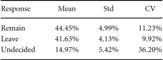
The analysis was done on the results of 168 opinion polls, which were conducted prior to the referendum that took place on 23rd June 2016. Out of the 168 polls, 155 of them also recorded how many people were undecided at the time. The data set was obtained online from(What UK thinks: EU2016), thefirst poll being taken on 1st September 2015 and the last one taken the day before the referendum. The mean, standard deviation(Std)and coefficient of variation(CV, defined as Std/Mean)for the polls is shown in table1; it can be seen that, according to the polls, the Remain campaign was leading, on average, by approximately 3% during the polling period. In addition, it can be seen that the CV, approximately 11% for Remain and 10% for Leave, is rather high, indicating that, according to the polls, the referendum result was far from certain. It is clear that the standard deviation for Undecided is high relative to its mean, giving rise to the very high CV, which is indicative of the volatility of the Undecided vote.

As a preliminary step, we test the statistical significance of the difference between Remain and Leave for each of the polls, using a 95% confidence interval for the difference between two proportions from the same

population(Seber2013, equation 3.4) (see also(Scott and Seber1983)and(Franklin2007)), given by

p p p p p p

n

1.96 , 1

1 2

1 2 1 2 2

-  + -

-ˆ ˆ ˆ ˆ ( ˆ ˆ ) ( )

wherepˆ₁is the Remain proportion, pˆ₂is the Leave proportion, andnis the sample size.

Overall, in 70 out of the 168 polls, i.e. 41.67%, the difference between Remain and Leave was significant. Furthermore, in 56 out of those 70 polls, i.e. 80% of the statistically significant polls, the proportion for Remain was larger than the proportion for Leave. Interestingly, when looking at all of the 168 polls, in 99 of these the proportion for Remain was larger than that for Leave, which is only 58.93% compared to the 80% for Remain in the significant polls. In the actual referendum 33,551,983 people voted, which was a massive turnout of 72.2% of the electorate. Out of these, 48.11% voted Remain and 51.89% voted Leave, which is a statistically significant result according to the test. Moreover, the difference between Leave and Remain was 3.78%, and the 95% confidence interval for the difference, i.e.,[3.75%, 3.81%], is very narrow.

We next divided the 168 polls into two equal groups, where thefirst 84 took place from September 2015 until the 22nd March 2016, and the second 84 took place from the 23rd of March 2016 until the day before the referendum. It transpired that for 41 out of thefirst group of polls, i.e. 48.81%, the difference between the Remain and Leave proportions was statistically significant, while for the second group it was significant for only 29 polls, i.e. 34.52%. Out of the 41 significant polls in thefirst group, Remain was leading in 36 polls, i.e. 87.80%, while, out of the 29 significant polls in the second group, Remain was leading in 19 polls, i.e. 65.52%. However, considering the overall poll results, whether significant or not, Remain was leading in 57 polls in thefirst group , i.e. 67.86%, whereas Remain was leading in only 42 polls in the second group, i.e. 50%. This indicates that, although, according to the polls, the gap between Remain and Leave was closing as the referendum approached, it was nevertheless quite likely that Remain would win thefinal vote.

We also tested whether the proportion of undecided voters during the polling period was significantly different from zero, using the 95% confidence interval for a single proportion(Seber2013, equation 2.4), known as Wald’s confidence interval, given by

p p p

n

1.96 1 , 2



-ˆ ˆ ( ˆ ) ( )

wherepˆis the Undecided proportion andnis the sample size.

In all of the 155 polls that recorded undecided voters, the proportion of undecided voters was significant. On average 14.97% of voters in these 155 polls indicated that their vote was undecided, and this vote could have potentially swayed these polls in either direction.

We then computed themean absolute errorsand theroot mean square errors(Chai and Draxler2014)for Remain and Leave compared to thefinal results. The mean absolute error(MAE)is given by

Table 1.Mean and standard deviation for the polls. Response Mean Std CV Remain 44.45% 4.99% 11.23% Leave 41.63% 4.13% 9.92% Undecided 14.97% 5.42% 36.20%

3

MAE p f

n , 3

i n

i

1

å

= =∣ - ∣ _{( )}

wherepiis the Remain or Leave proportion in theith poll,fis the Remain or Leave proportion of votes in the

actual referendum, andnis the number of polls. The root mean square error(RMSE)is given by

RMSE p f

n . 4

i n

i

1

2

å

= = ( - ) _{( )}

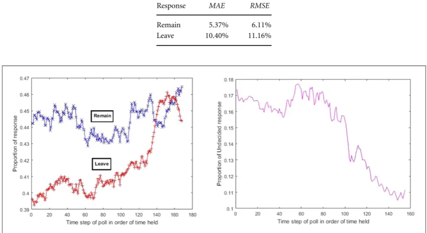
The results are shown in table2, where it can be seen that the errors for Leave are approximately twice as large as those for Remain. This is not surprising given thefinal, somewhat unexpected, result.

When analysing the data, it is also interesting to inspect the moving average(Chatfield1996)of the polls, as shown infigure1, in order to see any trend. In this case it is clear that, as the referendum date approached, the Leave vote was gaining traction and the proportion of Undecided votes was decreasing.

3. A random walk model for generating time series with application to poll results

Stochastic differential equations(SDEs) (Mackevicius2011, Evans2013)can provide effective generative models for time series. In particular, when the SDEs are‘mean reverting’(Hirsa and Neftci2014), as is the case here, they often possess stationary solutions thatfit various known distributions(Cobb1981, Bibbyet al2005). In our application, analysing poll results, the beta distribution(Gupta and Nadarajah2004)is a natural choice, since it isflexible, designed to model proportions due to its bounded support(Kotz and van Dorp2004), and is the conjugate prior of the binomial distribution. We also considered the gamma distribution(Johnsonet al1994), which is a reasonable choice given its relationship to the beta distribution(Leemis and McQueston2008). However, it only leads to an approximation of the bounded domain and, moreover, it is non-trivial to constrain it to a bounded domain. Generating beta distribution models using SDEs has applications in other domains, notably infinance(Taufer2007).

A typicalstochastic differential equation(SDE)takes the form

X X t X W

d t =m( t)d +s( t)d t, ( )5

whereXtis a random variable witht…0 a real number denoting time,μ(Xt)andσ(Xt)are known as thedriftand

diffusionfunctions, respectively, andWtis a Wiener process(also known as Brownian motion). Moreover, when

Xt m Xt , 6

m( )=q( - ) ( )

whereθ, therate parameter, is a positive constant andmis a constant representing the mean of the underlying stochastic diffusion process, the SDE has a stationary solution(Cobb1981). In addition, itsautocorrelation

Table 2.MAEandRMSEfor the polls. Response MAE RMSE

Remain 5.37% 6.11% Leave 10.40% 11.16%

Figure 1.Moving average with a centred sliding window of 25 time steps for the Remain and Leave(left), and Undecided(right)poll results.

4

functionis exponentially decreasing(Bibbyet al2005)and takes the form

t

exp(-q). ( )7

It was shown in(Cobb1981, Bibbyet al2005)that, if

m a 8

a b =

+ ( )

and

Xt 2 Xt 1 Xt , 9

2 s q a b = + -( ) ( ) ( )

then the marginal distribution of the stationary solution of the SDE is a beta distribution(Gupta and Nadarajah2004)with probability density function

x 1 1 x 1, 10

a b a b G +

G G

-a- b

-( )

( ) ( ) ( ) ( )

whereΓis the gamma function(Abramowitz and Stegun1972, 6.1).

Substituting(6)and(9)into(5), we obtain the SDE for a diffusion process with a marginal beta distribution in the form

X X t X X W

d t q t d 2 t 1 t d t. 11

a a b q a b = + - + + -⎛ ⎝ ⎜ ⎞ ⎠ ⎟ ( ) ( )

We note that several other forms formandσ2(Xt)also lead to well-known distributions(Cobb1981, Bibby

et al2005). Although we maintain that the SDE model we adopt is a natural one in our context, we note that a different model based on Markov chains, which also has a beta distribution as its stationary solution, has been presented in(Pacheco-Gonzalez and Stoyanov2008). In this Markov chain model, at any given time step, the movement in the time series may be up or down with a certain probability. Then the new position, in the interval between zero and one is determined according to some density function. Although promising, the results in

(Pacheco-Gonzalez and Stoyanov2008)are not as general as those of the SDE model, and depend on making a choice of parameters that would be difficult to determine from the data.

In reality, the continuous SDE model is an approximation of a discrete process described by a stochastic difference equation, wherexiis the discrete analogue of the random variableXtiat discrete timeti. Setting

x0=X0, the dynamics of the discrete process can be described by the difference equation

xi 1 q xi ti 1 2 xi 1 xi Wi 1, 12

a a b

q a b D =

+ - D + + - D

+ + + ⎛ ⎝ ⎜ ⎞ ⎠ ⎟ ( ) ( )

corresponding to(11), where

xi 1 xi 1 xi, 13

D + = + - ( )

ti 1 ti 1 ti, 14

D + = + - ( )

and

Wi 1 zi 1 ti 1, 15

D + = + D + ( )

wherezi+1is a normally distributed random variable with mean 0 and variance 1.

Using(12)to obtain a computational solution of(5)is known as theEuler-Maruyama method(Sauer2013), which is a general method for obtaining approximate numerical solutions to SDEs. We note that this method and various refinements of it are especially useful when analytic solutions do not exist(Iacus2008).

In our model of the polls, we assume that theith poll is conducted at timeti, whereti=i. Thus, in this case,

Δti+1in(14)and(15)is taken to be 1. The proportion of the poll respondents voting for a given outcome, for

example Remain, is represented byxi, where 0„xi„1.

4. Analysis of the Brexit polls considered as a random walk

To evaluate the model, we followed a similar approach to that taken in(Taufer2007). Wefirstfit a beta distribution to the marginal distribution of the time series induced by the poll results using the maximum likelihood method to obtain estimates forαandβ. We then used the Jensen-Shannon divergence, defined below, to measure the goodness offit. Lastly, wefit the autocorrelation function of the time series using least squares nonlinear regression to obtain an estimate forθ. All computations were carried out using the Matlab software package.

5

TheJensen-Shannon divergence(JSD) (Endres and Schindelin2003)is a nonparametric measure of the distance between two distributionsp=(pi)andq=(qi), wherei=1, 2,K,n. The formal definition of theJSD,

which is a symmetric version of the Kullback-Leibler divergence and is based on Shannon’s entropy(Cover and Thomas1991), is given by

JSD p p

p q q

q

p q

p q, 1

2 ln 2 ln 2

ln 2 , 16

i n

i

i

i i

i

i

i i

1

å

+ + +

= ⎛ ⎝

⎜ ⎞

⎠ ⎟

( ) ( )

where we use the convention that ifpi=0 orqi=0, or both,0 ln 0and0 ln 0 0( )are both defined to be 0.(The

factor2 ln 2is included to normalise theJSDto be between 0 and 1.)We observe that the JSD is equal to 0 whenp=q.

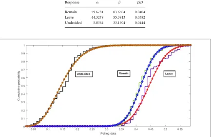
In table3we show the parameters of the beta distributionfitted by the maximum likelihood method, and the JSD between the empirical distribution of the time series of the poll results and thefitted beta distribution. The low JSD values indicate goodfits for all three responses. Infigure2we show a visual representation, here using cumulative distributionsto highlight the similarities between the empirical andfitted distributions. We note that the fact that the value of the JSD for Leave is somewhat higher is also noticeable fromfigure2.

In order to compute the rate parametersθof the sample autocorrelation function for the three responses, we

first smoothed the autocorrelation using a moving averagefilter with a centred sliding window of 5 lags. We then

fitted(7)to the smoothed values. The values obtained forθare shown in table4, together with the coefficient of determinationR2(Motulsky1995), the very high values of which indicate goodfits.(We note that usingR2as a goodness-of-fit measure for nonlinear least squares regression is somewhat controversial, although it has a natural interpretation as the comparison of a given model to the null model(Anderson-Sprecher1994).)

Table 3.Maximum likelihoodfitting of the beta distribution to the referendum polls.

Response α β JSD

Remain 59.6781 83.6604 0.0404 Leave 44.3278 55.3813 0.0582 Undecided 5.8364 33.1904 0.0444

Figure 2.Visual presentation of the cumulativefitted beta distributions.

Table 4.Exponential decay autocorrelation parameter of the referendum polls.

Response θ R2

Remain 0.9462 0.9716 Leave 0.7902 0.9393 Undecided 0.9963 0.9731

6

As a demonstration of the predictive power of the model, for each value ofi, we computed the 95% confidence interval for the difference between the proportions for theith and(i+1)th polls, using(12); accordingly, we replacedzi+1in(15)by±1.96. We used thefirst third of the polls for computing initial values for

the parametersαandβof the beta distribution, and the rate parameterθ. For the remaining two thirds of the polls and for each response, we next computed the difference between the proportion choosing that response in the poll and the corresponding proportion in the following poll. We then checked whether this difference was in the computed confidence interval. After each step we recomputed the values ofα,βandθusing all the polls up until the current one. The results are shown in table5, and it can be seen that the predictions for each response were within the appropriate confidence interval over 97% of the time.

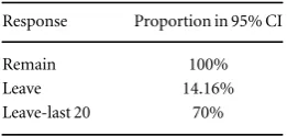
We also computed the difference between the actual result of the referendum and the current poll, to determine whether this difference was in the same confidence interval(this is equivalent to assuming that the following poll was the actual referendum). It turns out, as can be seen in table6, that the actual referendum result for Remain was within the predicted confidence intervals in all cases, while this was true for Leave only about 14% of the time. However, this percentage for Leave increases to 70% if only the last 20 polls are considered. Thus, even for the supposedly unpredictable referendum result, this is consistent with the adage that the later polls are more informative than the earlier ones.

5. Concluding remarks

We have proposed a generative stochastic differential equation model to analyse the time series of poll results; this possesses a stationary solution and the marginal distribution of the time series is a beta distribution. We provided empirical evidence that the model is a goodfit to the polls leading up to the Brexit referendum, and also provides good predictive power for the next step prediction task. We intend investigating other data sets for further validation of the model such as the analysis of polls leading up to a general election.

Acknowledgments

The authors would like to thank the reviewers for their constructive comments, which helped us to improve the paper.

ORCID iDs

Mark Levene https://orcid.org/0000-0001-8632-4732

References

Abramowitz M and Stegun I(ed)1972Handbook of Mathematical Functions with Formulas, Graphs and Mathematical tables(New York, NY: Dover)

Table 5.Percentages of the polls for which the following poll result is within the 95% con_fidence interval₍CI₎ relative to the next step prediction. Response Proportion in 95% CI Remain 100% Leave 98.23% Undecided 97.12%

Table 6.Percentages of the polls for which the actual referendum result is within the 95% confidence interval(CI) relative to the next step prediction. Response Proportion in 95% CI Remain 100% Leave 14.16% Leave-last 20 70%

7

Albert R and Barabási A-L 2002 Statistical mechanics of complex networksRev. Mod. Phys.7447_–97

Anderson-Sprecher R 1994 Model comparisons and R2_{The American Statistician48113–7}

Anuta D, Churchin J and Luo J 2017 Election bias: comparing polls and Twitter in the 2016 U.S. electionSocial and Information Networks ArchivearXiv:1701.06232v1[cs.SI]

Barabási A-L 2016Network Science(Cambridge, UK: Cambridge University Press)

Bentley A and Ormerod P 2011 Agents, intelligence, and social atomsCreating Consilience: Integrating the Sciences and the Humanitiesed E Slingerland and M Collard(New York, NY: Oxford University Press)pp 205–22

Bibby B, Skovgaard I and Sørensen M 2005 Diffusion-type models with given marginal distribution and autocorrelation functionBernoulli 11191–220

Bohannon J 2017 The pulse of the people: can internet data outdo costly and unreliable polls in predicting election outcomes?Science355

470–2

Castellano C, Fortunato S and Loreto V 2009 Statistical physics of social dynamicsRev. Mod. Phys.81591–646

Chai T and Draxler R 2014 Root mean square error(RMSE)or mean absolute error(MAE)? - Arguments against avoiding RMSE in the literatureGeoscientific Model Development71247–50

Chatfield C 1996The Analysis of Time Series: An Introduction, Text in Statistical Science5th edn(London: chapman & Hall)

Cobb L 1981 Stochastic differential equations for the social sciencesMathematical Frontiers of the Social and Policy Sciencesed L Cobb and R Thral(Bolder, CO: Westview Press)ch2

Conte R and Paolucci M 2014 On agent-based modeling and computational social scienceFrontiers in Physiology59ppArticle 668 Converse P and Traugott M 1986 Assessing the accuracy of polls and surveysScience2341094_–8

Cover T and Thomas J 1991Elements of Information Theory₍Chichester: John Wiley & Sons₎Wiley Series in Telecommunications Eknoyan G 2008 Adolphe Quetelet(1796–1874)- the average man and indices of obesityNephrology Dialysis Transplantation2347–51

Endres D and Schindelin J 2003 A new metric for probability distributionsIEEE Trans. Inf. Theory491858–60

Evans L 2013An Introduction to Stochastic Differential equations(Providence, RI: American Mathematical Society)

Fenner T, Kaufmann E, Levene M and Loizou G 2017 A multiplicative process for generating a beta-like survival function with application to the UK 2016 EU referendum resultsInt. J. Mod. Phys.C28175013214 pages

Fenner T, Levene M and Loizou G 2015 A stochastic evolutionary model for capturing human dynamicsJournal of Statistical Mechanics: Theory and Experiment2015P08015

Fenner T, Levene M and Loizou G 2018 A multiplicative process for generating the rank-order distribution of UK election resultsQuality & Quantity521069–79

Franklin C 2007 The margin of error for differences in polls Seehttps://abcnews.go.com/images/PollingUnit/MOEFranklin.pdf. Galam S 2008 Sociophysics: a review of Galam modelsJournal of Modern PhysicsC19409–40

Goodwin M and Heath O 2016 The 2016 referendum, Brexit and the left behind: an aggregate-level analysis of the resultThe Political Quarterly87323–32

Guolo A and Varin C 2014 Beta regression for time series analysis of bounded data, with application to Canada Googleflu trendsThe Annals of Applied Statistics874–88

Gupta A and Nadarajah S₍ed₎2004Handbook of Beta Distribution and its Applications₍New York, NY: Marcel Dekker₎Statistics: Textbooks and Monographs

Hair J Jr., Black W, Babin B and Anderson R 2014Multivariate Data Analysis7th edn₍Harlow, UK: Pearson Education₎ Hirsa A and Neftci S 2014An Introduction to the Mathematics of Financial Derivatives3rd edn₍San Diego, CA: Academic₎

Iacus S 2008Simulation and Inference for Stochastic Differential equations: With R Examples(Berlin: Springer)Springer Series in Statistics Johnson N, Kotz S and Balkrishnan N 1994Continuous Univariate Distributions, vol 1, Wiley Series in Probability and Mathematical Statistics

2nd edn(New York, NY: Wiley)pp 337–414 ch 17 Gamma distributions

Juhl R, Møller J, Jørgensen J and Madsen H 2016 Modeling and prediction using stochastic differential equationsPrediction Methods for Blood Glucose Concentration: Design, Use and Evaluation, Lecture Notes in Bioengineeringed H Kirchsteigeret al(Cham, Switzerland: Springer)pp 183–209

Kleinbaum D and Klein M 2012Survival Analysis, A Self-Learning Text3rd edn(New York, NY: Springer Science+Business Media, LLC) Kononovicius A 2017 Empirical analysis and agent-based modeling of the Lithuanian parliamentary electionsComplexity20177354642

Kotz S and van Dorp J 2004Beyond Beta: Other Continuous Families of Distributions with Bounded Support and Applications(Singapore: World Scientific)

Leemis L and McQueston J 2008 Univariate distribution relationshipsThe American Statistician6245–53

Liu B 2015Sentiment Analysis: Mining Opinions, Sentiments, and Emotions(Cambridge, UK: Cambridge University Press)

Mackevicius V 2011Introduction to Stochastic Analysis: Integrals and Differential equations(London, UK and Hoboken NJ: ISTE Ltd and John Wiley & Sons)Applied Stochastic Methods Series

Martínez-Mekler G, Alvarez Martínez R, Beltrán del Rio M, Mansilla R, Miramontes P and Cocho G 2009 Universality of rank-ordering distributions in the arts and sciencesPLoS ONE4e4791

Motulsky H 1995Intuitive Biostatistics₍Oxford: Oxford University Press₎

O’Connor B, Balasubramanyan R, Routledge B and Smith N 2010 From tweets to polls: Linking text sentiment to public opinion time series

Proc. of the Fourth AAAI Conf. on Weblogs and Social Media (Washington, DC)pp 122–9

Pacheco-Gonzalez C and Stoyanov J 2008 A class of Markov chains with beta ergodic distributionsThe Mathematical Scientist33110–9 Sauer T 2013 Computational solution of stochastic differential equationsWiley Interdisciplinary Reviews: Computational Statistics5362–71

Scott A and Seber G 1983 Difference of proportions from the same surveyThe American Statistician37319–20 Seber G 2013Statistical Models for Proportions and Probabilities(Heidelberg: Springer)SpringerBriefs in Statistics Sen P and Chakrabarti B 2014Sociophysics: An Introduction(Oxford: Oxford University Press)

Simon H 1955 On a class of skew distribution functionsBiometrika42425–40

Sirbu A, Loreto V, Servedio V and Tria F 2017 Opinion dynamics: models, extensions and external effectŝ Participatory Sensing, Opinions and Collective Awareness(Understanding Complex Systems)ed V Loretoet al(Cham, Switzerland: Springer International Publishing) pp 363–401 ch17

Sornette D, Knopoff L, Kagan Y and Vanneste C 1996 Rank-ordering statistics of extreme events: application to the distribution of large earthquakesJ. Geophys. Res.10113–883

Stewart J 1950 The development of social physicsAm. J. Phys.18239–53

Taufer E 2007 Modelling stylized features in default ratesApplied Stochastic Models in Business and Industry2373–82

2016 What UK thinks: EU . UK poll resultshttp://whatukthinks.org/eu/questions/ should-the-united-kingdom-remain-a-member-of-the-eu-or-leave-the-eu.

8

Wlezien C and Erikson R 2002 The timeline of presidential election campaignsThe Journal of Politics64969_–93

Wlezien C, Jennings W and Erikson R 2017 The_‘timeline_’method of studying electoral dynamicsElectoral Studies4845_–56

9